Distributed Arithmetic
Distributed Arithmetic
Consider calculating the following expression:
y=N∑i=1cixiy=∑i=1Ncixi
where the cici coefficients are fixed-valued and xixi represents the inputs of the multiply-and-accumulate operation. Assume that these inputs are in two’s complement format and are represented by b+1 bits. Moreover, assume that they are scaled and are less than 1 in magnitude. To keep things simple, we’ll consider the above equation for N=3. Hence,
y=c1x1+c2x2+c3x3y=c1x1+c2x2+c3x3
Equation 1
Since the inputs are in two’s complement format, we can write
x1=−x1,0+b∑j=1x1,j2−jx1=−x1,0+∑j=1bx1,j2−j
x2=−x2,0+b∑j=1x2,j2−jx2=−x2,0+∑j=1bx2,j2−j
x3=−x3,0+b∑j=1x3,j2−jx3=−x3,0+∑j=1bx3,j2−j
where x1,0x1,0 is the sign bit of x1x1 and x1,jx1,j is the jth bit to the right of the sign bit. The same notation is used for x2x2 and x3x3. If you need help with deriving these equations, read the section entitled “An Important Feature of the Two’s Complement Representation” in my article, "Multiplication Examples Using the Fixed-Point Representation" and note that we have assumed |xi|<1|xi|<1.
Substituting our last three equations into Equation 1 gives
y=−x1,0c1+x1,1c1×2−1+⋯+x1,bc1×2−b−x2,0c2+x2,1c2×2−1+⋯+x2,bc2×2−b−x3,0c3+x3,1c3×2−1+⋯+x3,bc3×2−by=−x1,0c1+x1,1c1×2−1+⋯+x1,bc1×2−b−x2,0c2+x2,1c2×2−1+⋯+x2,bc2×2−b−x3,0c3+x3,1c3×2−1+⋯+x3,bc3×2−b
Equation 2
How can we use a LUT to efficiently implement these calculations?
For now, let’s ignore the 2−j2−j terms of Equation 2 and look at this equation as a summation of some columns rather than a summation of some rows. For example, the second column of Equation 2 is
y1=x1,1c1+x2,1c2+x3,1c3y1=x1,1c1+x2,1c2+x3,1c3
How many distinct values are there for this expression? Note that x1,1x1,1, x2,1x2,1, and x3,1x3,1 are one-bit values. Hence, y1y1 can have only eight distinct values as given in Table 1 below:
Table 1
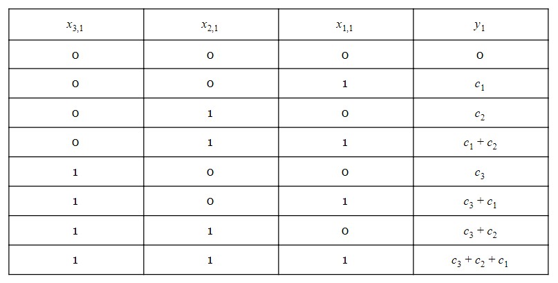
Ignoring the 2−b2−b term of the last column, we have
yb=x1,bc1+x2,bc2+x3,bc3yb=x1,bc1+x2,bc2+x3,bc3
Again, we can only have the eight distinct values of Table 1. As you can see, the columns of Equation 2 involve calculating the function given by Table 1 (provided that we ignore the minus sign of the first column and the 2−j2−j terms). Instead of repeatedly calculating this function, we can pre-calculate the values of y1y1 and store them in a LUT, as shown in the following block diagram:
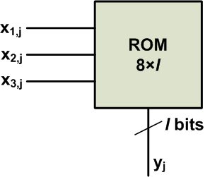
Figure 1
As shown in the figure, the jth bit of all the input signals, x1x1, x2x2, x3x3, will be applied to the LUT, and the output will be yjyj. The output of the ROM is represented by l bits. l must be large enough to store the values of Table 1 without overflow.
Now that the LUT is responsible for producing the yjyj terms, we can rewrite Equation 2 as
y=−y0+2−1y1+2−2y2+⋯+2−byby=−y0+2−1y1+2−2y2+⋯+2−byb
Therefore, we need to take the 2−j2−j terms into account and note that the first term must be subtracted from the other terms.
Let’s assume that we are using only five bits to represent the xixi signals, i.e., b=4b=4. Hence,
y=−y0+2−1y1+2−2y2+2−3y3+2−4y4y=−y0+2−1y1+2−2y2+2−3y3+2−4y4
By repeatedly factoring 2−12−1, we can rewrite the above equation as
y=−y0+2−1(y1+2−1(y2+2−1(y3+2−1(y4+0))))y=−y0+2−1(y1+2−1(y2+2−1(y3+2−1(y4+0))))
Note that a zero is added to the innermost parentheses to further clarify the pattern that exists. The multiply-and-add operation is now written as a repeated pattern consisting of a summation and a multiplication by 2−12−1. We know that multiplication by 2−12−1 can be implemented by a one-bit shift to the right. Therefore, we can use the ROM shown in Figure 1 along with a shift register and an adder/subtractor to implement the above equation. The simplified block diagram is shown in Figure 2.
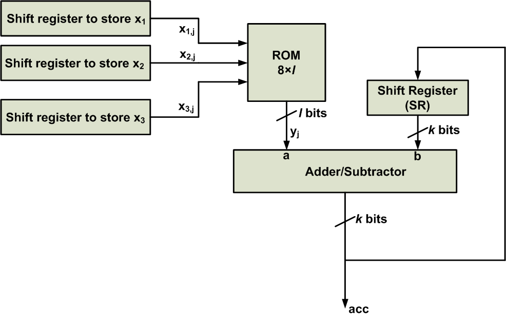
Figure 2
At the beginning of the calculations, the shift register SR is reset to zero and the other shift registers are loaded with the appropriate inputs. Then, the registers x1x1, x2x2, and x3x3 apply x1,4x1,4, x2,4x2,4, and x3,4x3,4 to the ROM. Hence, the adder will produce acc=a+b=y4+0=y4acc=a+b=y4+0=y4. This value will be stored in the SR, and a one-bit shift will be applied to take the 2−12−1 term into account. (As we’ll see in a minute, the output of the adder/subtractor will generate the final result of the algorithm by gradually accumulating the partial results. That’s why we’ve used “acc”, which stands for accumulator, to represent the output of the adder/subtractor.)
So far, 2−1(y4+0)2−1(y4+0) has been generated at the output of the SR register. Next, the input registers will apply x1,3x1,3, x2,3x2,3, and x3,3x3,3 to the ROM. Hence, the adder will produce acc=a+b=y3+2−1(y4+0)acc=a+b=y3+2−1(y4+0). Again, this value will be stored in the SR and a one-bit shift will be applied to take the 2−12−1 term into account, which gives 2−1(y3+2−1(y4+0))2−1(y3+2−1(y4+0)). In a similar manner, the sum and shift operations will be repeated for the next terms, except that for the last term, the adder/subtractor will be in the subtract mode.
Note that the number of shift-and-add operations in Figure 2 does not depend on the number of input signals N. The number of inputs affects only the size of the ROM’s address input. This is a great advantage of the DA technique over a conventional implementation of a multiply-and-add operation, i.e., an implementation in which partial products are generated and added together. However, a large N can lead to a slow ROM and reduce the efficiency of the technique.
In the DA architecture, the number of shift-and-add operations depends on the number of bits used to represent the input signals, which in turn depends on the precision that the system requires.
Conclusion
DA recognizes some frequently used values of a multiply-and-accumulate operation, pre-computes these values and stores them in a lookup-table (LUT). Reading these stored values from ROM rather than calculating them leads to an efficient implementation. It should be noted that the DA method is applicable only to cases where the multiply-and-accumulate operation involves fixed coefficients.
Last updated