Pytorch
Production Ready
Transition seamlessly between eager and graph modes with TorchScript, and accelerate the path to production with TorchServe.
Distributed Training
Scalable distributed training and performance optimization in research and production is enabled by the torch.distributed backend.
Robust Ecosystem
A rich ecosystem of tools and libraries extends PyTorch and supports development in computer vision, NLP and more.
Cloud Support
PyTorch is well supported on major cloud platforms, providing frictionless development and easy scaling.
Explore a rich ecosystem of libraries, tools, and more to support development.
Community
Join the PyTorch developer community to contribute, learn, and get your questions answered.
Learn the Basics
Familiarize yourself with PyTorch concepts and modules. Learn how to load data, build deep neural networks, train and save your models in this quickstart guide.
PyTorch Recipes
Bite-size, ready-to-deploy PyTorch code examples.
Examples of PyTorch
A set of examples around pytorch in Vision, Text, Reinforcement Learning, etc.
PyTorch Cheat Sheet
Quick overview to essential PyTorch elements.
Tutorials on GitHub
Access PyTorch Tutorials from GitHub.
Run Tutorials on Google Colab
Learn how to copy tutorial data into Google Drive so that you can run tutorials on Google Colab.
We’ve added a new feature to tutorials that allows users to open the notebook associated with a tutorial in Google Colab. You may need to copy data to your Google drive account to get the more complex tutorials to work.
In this example, we’ll demonstrate how to change the notebook in Colab to work with the Chatbot Tutorial. To do this, you’ll first need to be logged into Google Drive. (For a full description of how to access data in Colab, you can view their example notebook here.)
To get started open the Chatbot Tutorial in your browser.
At the top of the page click Run in Google Colab.
The file will open in Colab.
If you select Runtime, and then Run All, you’ll get an error as the file can’t be found.
To fix this, we’ll copy the required file into our Google Drive account.
Log into Google Drive.
In Google Drive, make a folder named data, with a subfolder named cornell.
Visit the Cornell Movie Dialogs Corpus and download the ZIP file.
Unzip the file on your local machine.
Copy the files movie_lines.txt and movie_conversations.txt to the data/cornell folder that you created in Google Drive.
Now we’ll need to edit the file in_ _Colab to point to the file on Google Drive.
In Colab, add the following to top of the code section over the line that begins corpus_name:
from google.colab import drive drive.mount('/content/gdrive')
Change the two lines that follow:
Change the corpus_name value to “cornell”.
Change the line that begins with corpus to this:
corpus = os.path.join("/content/gdrive/My Drive/data", corpus_name)
We’re now pointing to the file we uploaded to Drive.
Now when you click the Run cell button for the code section, you’ll be prompted to authorize Google Drive and you’ll get an authorization code. Paste the code into the prompt in Colab and you should be set.
Rerun the notebook from the Runtime / Run All menu command and you’ll see it process. (Note that this tutorial takes a long time to run.)
Hopefully this example will give you a good starting point for running some of the more complex tutorials in Colab. As we evolve our use of Colab on the PyTorch tutorials site, we’ll look at ways to make this easier for users.
Note
Click here to download the full example code
torchaudio implements feature extractions commonly used in the audio domain. They are available in torchaudio.functional and torchaudio.transforms.
functional implements features as standalone functions. They are stateless.
transforms implements features as objects, using implementations from functional and torch.nn.Module. Because all transforms are subclasses of torch.nn.Module, they can be serialized using TorchScript.
For the complete list of available features, please refer to the documentation. In this tutorial, we will look into converting between the time domain and frequency domain (Spectrogram, GriffinLim, MelSpectrogram).
# When running this tutorial in Google Colab, install the required packages # with the following. # !pip install torchaudio librosa
import torch import torchaudio import torchaudio.functional as F import torchaudio.transforms as T
print(torch.__version__) print(torchaudio.__version__)
Out:
1.10.0+cu102 0.10.0+cu102
Preparing data and utility functions (skip this section)
#@title Prepare data and utility functions. {display-mode: "form"} #@markdown #@markdown You do not need to look into this cell. #@markdown Just execute once and you are good to go. #@markdown #@markdown In this tutorial, we will use a speech data from [VOiCES dataset](https://iqtlabs.github.io/voices/), which is licensed under Creative Commos BY 4.0.
#------------------------------------------------------------------------------- # Preparation of data and helper functions. #-------------------------------------------------------------------------------
import os import requests
import librosa import matplotlib.pyplot as plt from IPython.display import Audio, display
_SAMPLE_DIR = "_sample_data"
SAMPLE_WAV_SPEECH_URL = "https://pytorch-tutorial-assets.s3.amazonaws.com/VOiCES_devkit/source-16k/train/sp0307/Lab41-SRI-VOiCES-src-sp0307-ch127535-sg0042.wav" SAMPLE_WAV_SPEECH_PATH = os.path.join(_SAMPLE_DIR, "speech.wav")
os.makedirs(_SAMPLE_DIR, exist_ok=True)
def _fetch_data(): uri = [ (SAMPLE_WAV_SPEECH_URL, SAMPLE_WAV_SPEECH_PATH), ] for url, path in uri: with open(path, 'wb') as file_: file_.write(requests.get(url).content)
_fetch_data()
def _get_sample(path, resample=None): effects = [ ["remix", "1"] ] if resample: effects.extend([ ["lowpass", f"{resample // 2}"], ["rate", f'{resample}'], ]) return torchaudio.sox_effects.apply_effects_file(path, effects=effects)
def get_speech_sample(*, resample=None): return _get_sample(SAMPLE_WAV_SPEECH_PATH, resample=resample)
def print_stats(waveform, sample_rate=None, src=None): if src: print("-" * 10) print("Source:", src) print("-" * 10) if sample_rate: print("Sample Rate:", sample_rate) print("Shape:", tuple(waveform.shape)) print("Dtype:", waveform.dtype) print(f" - Max: {waveform.max().item():6.3f}") print(f" - Min: {waveform.min().item():6.3f}") print(f" - Mean: {waveform.mean().item():6.3f}") print(f" - Std Dev: {waveform.std().item():6.3f}") print() print(waveform) print()
def plot_spectrogram(spec, title=None, ylabel='freq_bin', aspect='auto', xmax=None): fig, axs = plt.subplots(1, 1) axs.set_title(title or 'Spectrogram (db)') axs.set_ylabel(ylabel) axs.set_xlabel('frame') im = axs.imshow(librosa.power_to_db(spec), origin='lower', aspect=aspect) if xmax: axs.set_xlim((0, xmax)) fig.colorbar(im, ax=axs) plt.show(block=False)
def plot_waveform(waveform, sample_rate, title="Waveform", xlim=None, ylim=None): waveform = waveform.numpy()
num_channels, num_frames = waveform.shape time_axis = torch.arange(0, num_frames) / sample_rate
figure, axes = plt.subplots(num_channels, 1) if num_channels == 1: axes = [axes] for c in range(num_channels): axes[c].plot(time_axis, waveform[c], linewidth=1) axes[c].grid(True) if num_channels > 1: axes[c].set_ylabel(f'Channel {c+1}') if xlim: axes[c].set_xlim(xlim) if ylim: axes[c].set_ylim(ylim) figure.suptitle(title) plt.show(block=False)
def play_audio(waveform, sample_rate): waveform = waveform.numpy()
num_channels, num_frames = waveform.shape if num_channels == 1: display(Audio(waveform[0], rate=sample_rate)) elif num_channels == 2: display(Audio((waveform[0], waveform[1]), rate=sample_rate)) else: raise ValueError("Waveform with more than 2 channels are not supported.")
def plot_mel_fbank(fbank, title=None): fig, axs = plt.subplots(1, 1) axs.set_title(title or 'Filter bank') axs.imshow(fbank, aspect='auto') axs.set_ylabel('frequency bin') axs.set_xlabel('mel bin') plt.show(block=False)
def plot_pitch(waveform, sample_rate, pitch): figure, axis = plt.subplots(1, 1) axis.set_title("Pitch Feature") axis.grid(True)
end_time = waveform.shape[1] / sample_rate time_axis = torch.linspace(0, end_time, waveform.shape[1]) axis.plot(time_axis, waveform[0], linewidth=1, color='gray', alpha=0.3)
axis2 = axis.twinx() time_axis = torch.linspace(0, end_time, pitch.shape[1]) ln2 = axis2.plot( time_axis, pitch[0], linewidth=2, label='Pitch', color='green')
axis2.legend(loc=0) plt.show(block=False)
def plot_kaldi_pitch(waveform, sample_rate, pitch, nfcc): figure, axis = plt.subplots(1, 1) axis.set_title("Kaldi Pitch Feature") axis.grid(True)
end_time = waveform.shape[1] / sample_rate time_axis = torch.linspace(0, end_time, waveform.shape[1]) axis.plot(time_axis, waveform[0], linewidth=1, color='gray', alpha=0.3)
time_axis = torch.linspace(0, end_time, pitch.shape[1]) ln1 = axis.plot(time_axis, pitch[0], linewidth=2, label='Pitch', color='green') axis.set_ylim((-1.3, 1.3))
axis2 = axis.twinx() time_axis = torch.linspace(0, end_time, nfcc.shape[1]) ln2 = axis2.plot( time_axis, nfcc[0], linewidth=2, label='NFCC', color='blue', linestyle='--')
lns = ln1 + ln2 labels = [l.get_label() for l in lns] axis.legend(lns, labels, loc=0) plt.show(block=False)
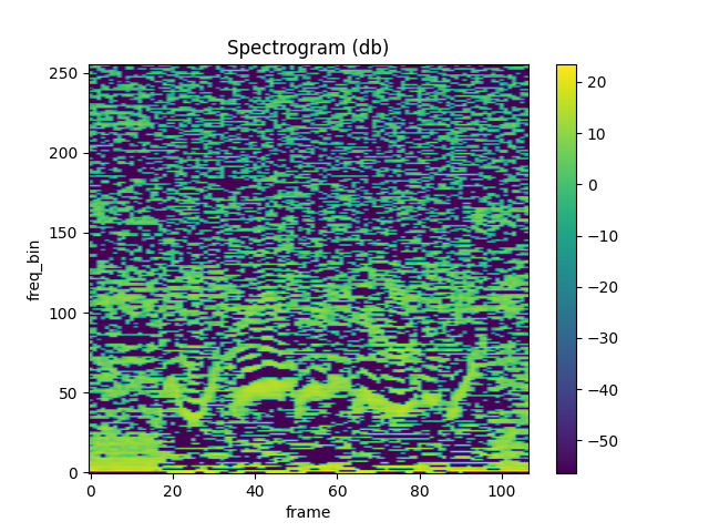
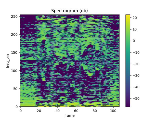
Spectrogram
To get the frequency make-up of an audio signal as it varies with time, you can use Spectrogram.
waveform, sample_rate = get_speech_sample()
n_fft = 1024 win_length = None hop_length = 512
# define transformation spectrogram = T.Spectrogram( n_fft=n_fft, win_length=win_length, hop_length=hop_length, center=True, pad_mode="reflect", power=2.0, ) # Perform transformation spec = spectrogram(waveform)
print_stats(spec) plot_spectrogram(spec[0], title='torchaudio')
Out:
Shape: (1, 513, 107) Dtype: torch.float32
Max: 4000.533
Min: 0.000
Mean: 5.726
Std Dev: 70.301
tensor([[[7.8743e+00, 4.4462e+00, 5.6781e-01, ..., 2.7694e+01, 8.9546e+00, 4.1289e+00], [7.1094e+00, 3.2595e+00, 7.3520e-01, ..., 1.7141e+01, 4.4812e+00, 8.0840e-01], [3.8374e+00, 8.2490e-01, 3.0779e-01, ..., 1.8502e+00, 1.1777e-01, 1.2369e-01], ..., [3.4708e-07, 1.0604e-05, 1.2395e-05, ..., 7.4090e-06, 8.2063e-07, 1.0176e-05], [4.7173e-05, 4.4329e-07, 3.9444e-05, ..., 3.0622e-05, 3.9735e-07, 8.1572e-06], [1.3221e-04, 1.6440e-05, 7.2536e-05, ..., 5.4662e-05, 1.1663e-05, 2.5758e-06]]])
GriffinLim
To recover a waveform from a spectrogram, you can use GriffinLim.
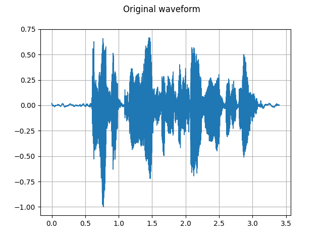
torch.random.manual_seed(0) waveform, sample_rate = get_speech_sample() plot_waveform(waveform, sample_rate, title="Original") play_audio(waveform, sample_rate)
n_fft = 1024 win_length = None hop_length = 512
spec = T.Spectrogram( n_fft=n_fft, win_length=win_length, hop_length=hop_length, )(waveform)
griffin_lim = T.GriffinLim( n_fft=n_fft, win_length=win_length, hop_length=hop_length, ) waveform = griffin_lim(spec)
plot_waveform(waveform, sample_rate, title="Reconstructed") play_audio(waveform, sample_rate)
Out:
<IPython.lib.display.Audio object> <IPython.lib.display.Audio object>
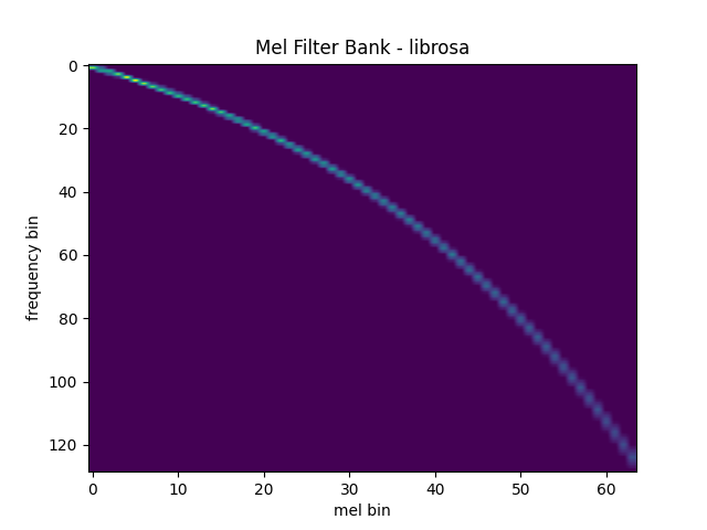
Mel Filter Bank
torchaudio.functional.create_fb_matrix generates the filter bank for converting frequency bins to mel-scale bins.
Since this function does not require input audio/features, there is no equivalent transform in torchaudio.transforms.
n_fft = 256 n_mels = 64 sample_rate = 6000
mel_filters = F.create_fb_matrix( int(n_fft // 2 + 1), n_mels=n_mels, f_min=0., f_max=sample_rate/2., sample_rate=sample_rate, norm='slaney' ) plot_mel_fbank(mel_filters, "Mel Filter Bank - torchaudio")

Comparison against librosa
For reference, here is the equivalent way to get the mel filter bank with librosa.
mel_filters_librosa = librosa.filters.mel( sample_rate, n_fft, n_mels=n_mels, fmin=0., fmax=sample_rate/2., norm='slaney', htk=True, ).T
plot_mel_fbank(mel_filters_librosa, "Mel Filter Bank - librosa")
mse = torch.square(mel_filters - mel_filters_librosa).mean().item() print('Mean Square Difference: ', mse)
Out:
Mean Square Difference: 3.795462323290159e-17
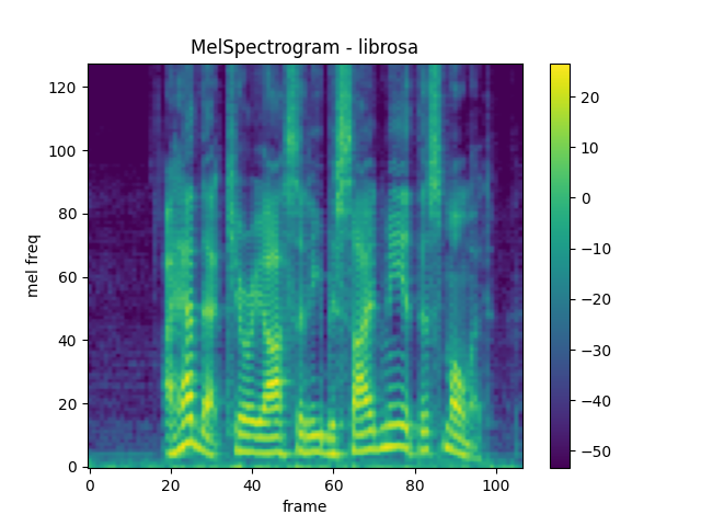
MelSpectrogram
Generating a mel-scale spectrogram involves generating a spectrogram and performing mel-scale conversion. In torchaudio, MelSpectrogram provides this functionality.
waveform, sample_rate = get_speech_sample()
n_fft = 1024 win_length = None hop_length = 512 n_mels = 128
mel_spectrogram = T.MelSpectrogram( sample_rate=sample_rate, n_fft=n_fft, win_length=win_length, hop_length=hop_length, center=True, pad_mode="reflect", power=2.0, norm='slaney', onesided=True, n_mels=n_mels, mel_scale="htk", )
melspec = mel_spectrogram(waveform) plot_spectrogram( melspec[0], title="MelSpectrogram - torchaudio", ylabel='mel freq')

Comparison against librosa
For reference, here is the equivalent means of generating mel-scale spectrograms with librosa.
melspec_librosa = librosa.feature.melspectrogram( waveform.numpy()[0], sr=sample_rate, n_fft=n_fft, hop_length=hop_length, win_length=win_length, center=True, pad_mode="reflect", power=2.0, n_mels=n_mels, norm='slaney', htk=True, ) plot_spectrogram( melspec_librosa, title="MelSpectrogram - librosa", ylabel='mel freq')
mse = torch.square(melspec - melspec_librosa).mean().item() print('Mean Square Difference: ', mse)
Out:
Mean Square Difference: 1.17573561997375e-10
MFCC
waveform, sample_rate = get_speech_sample()
n_fft = 2048 win_length = None hop_length = 512 n_mels = 256 n_mfcc = 256
mfcc_transform = T.MFCC( sample_rate=sample_rate, n_mfcc=n_mfcc, melkwargs={ 'n_fft': n_fft, 'n_mels': n_mels, 'hop_length': hop_length, 'mel_scale': 'htk', } )
mfcc = mfcc_transform(waveform)
plot_spectrogram(mfcc[0])

Comparing against librosa
melspec = librosa.feature.melspectrogram( y=waveform.numpy()[0], sr=sample_rate, n_fft=n_fft, win_length=win_length, hop_length=hop_length, n_mels=n_mels, htk=True, norm=None)
mfcc_librosa = librosa.feature.mfcc( S=librosa.core.spectrum.power_to_db(melspec), n_mfcc=n_mfcc, dct_type=2, norm='ortho')
plot_spectrogram(mfcc_librosa)
mse = torch.square(mfcc - mfcc_librosa).mean().item() print('Mean Square Difference: ', mse)
Out:
Mean Square Difference: 4.258112085153698e-08
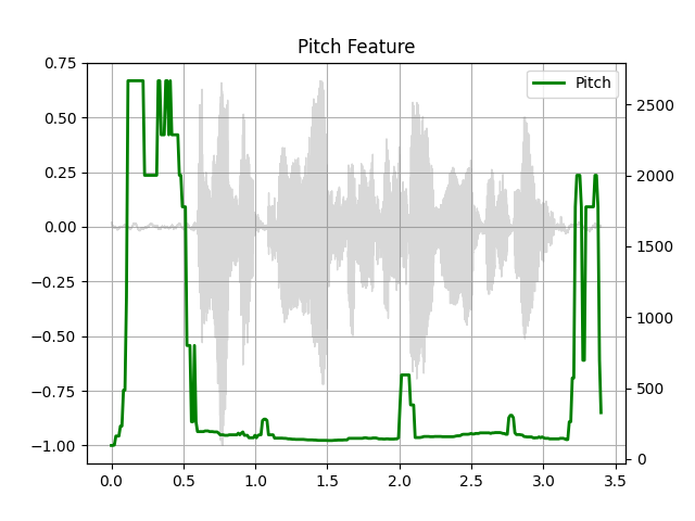
Pitch
waveform, sample_rate = get_speech_sample()
pitch = F.detect_pitch_frequency(waveform, sample_rate) plot_pitch(waveform, sample_rate, pitch) play_audio(waveform, sample_rate)
Out:
<IPython.lib.display.Audio object>
Kaldi Pitch (beta)
Kaldi Pitch feature [1] is a pitch detection mechanism tuned for automatic speech recognition (ASR) applications. This is a beta feature in torchaudio, and it is available only in functional.
A pitch extraction algorithm tuned for automatic speech recognition
Ghahremani, B. BabaAli, D. Povey, K. Riedhammer, J. Trmal and S. Khudanpur
2014 IEEE International Conference on Acoustics, Speech and Signal Processing (ICASSP), Florence, 2014, pp. 2494-2498, doi: 10.1109/ICASSP.2014.6854049. [abstract], [paper]
waveform, sample_rate = get_speech_sample(resample=16000)
pitch_feature = F.compute_kaldi_pitch(waveform, sample_rate) pitch, nfcc = pitch_feature[..., 0], pitch_feature[..., 1]
plot_kaldi_pitch(waveform, sample_rate, pitch, nfcc) play_audio(waveform, sample_rate)
Out:
<IPython.lib.display.Audio object>
Total running time of the script: ( 0 minutes 6.007 seconds)
Gallery generated by Sphinx-Gallery
Last updated