
Audio
Fast Fourier Transform
Visualizing the Discrete Fourier Transform
A couple of years ago I suggested a way of thinking about how the Discrete Fourier Transform works, based on Stuart Riffle's elegant colour-coding of the equation:
(Sadly, Stuart's original post describing the equation has been lost to bitrot, and can't even be found in the Wayback Machine.) My contribution was the following analogy:
Imagine an enormous speaker, mounted on a pole, playing a repeating sound. The speaker is so large, you can see the cone move back and forth with the sound. Mark a point on the cone, and now rotate the pole. Trace the point from an above-ground view, if the resulting squiggly curve is off-center, then there is frequency corresponding the pole's rotational frequency represented in the sound.
Dr Bill Connelly from Australia National University has created an interactive simulation of the analogy. Here, the sound from the speaker is a chord of two tones: just enter their frequency and amplitude, and see how the DFT is calculated from the analysis of the rotation:
Discrete Fast Fourier Transform
Frequency and the fast Fourier transform
If you want to find the secrets of the universe, think in terms of energy, frequency and vibration.
— Nikola Tesla
This chapter was written in collaboration with SW's father, PW van der Walt.
Introducing frequency
We'll start by setting up some plotting styles and importing the usual suspects:
The discretediscrete Fourier transform (DFT) is a mathematical technique to convert temporal or spatial data into frequency domain data. Frequency is a familiar concept, due to its colloquial occurrence in the English language: the lowest notes your headphones can rumble out are around 20 Hertz, whereas middle C on a piano lies around 261.6 Hertz. Hertz (Hz), or oscillations per second, in this case literally refers to the number of times per second at which the membrane inside the headphone moves to-and-fro. That, in turn, creates compressed pulses of air which, upon arrival at your eardrum, induces a vibration at the same frequency. So, if you take a simple periodic function, $\sin(10 \times 2 \pi t)$, you can view it as a wave:
Or you can equivalently think of it as a repeating signal of frequency 10 Hertz (it repeats once every $1/10$ seconds—a length of time we call its period). Although we naturally associate frequency with time, it can equally well be applied to space. E.g., a photo of a textile patterns exhibits high spatial frequency, whereas the sky or other smooth objects have low spatial frequency.
Let us now examine our sinusoid through application of the discrete Fourier transform:
We see that the output of the FFT is a one-dimensional array of the same shape as the input, containing complex values. All values are zero, except for two entries. Traditionally, we visualize the magnitude of the result as a stem plot, in which the height of each stem corresponds to the underlying value.
(We explain why you see positive and negative frequencies later on in the sidebox titled "Discrete Fourier transforms". You may also refer to that section for a more in-depth overview of the underlying mathematics.)
The Fourier transform takes us from the time to the frequency domain, and this turns out to have a massive number of applications. The fast Fourier transform is an algorithm for computing the discrete Fourier transform; it achieves its high speed by storing and re-using results of computations as it progresses.
In this chapter, we examine a few applications of the discrete Fourier transform to demonstrate that the FFT can be applied to multidimensional data (not just 1D measurements) to achieve a variety of goals.
Illustration: a birdsong spectrogram
Let's start with one of the most common applications, converting a sound signal (consisting of variations of air pressure over time) to a spectrogram. You might have seen spectrograms on your music player's equalizer view, or even on an old-school stereo.

Listen to the following snippet of nightingale birdsong (released under CC BY 4.0 at http://www.orangefreesounds.com/nightingale-sound/):
If you are reading the paper version of this book, you'll have to use your imagination! It goes something like this: chee-chee-woorrrr-hee-hee cheet-wheet-hoorrr-chi rrr-whi-wheo-wheo-wheo-wheo-wheo-wheo.
Since we realise that not everyone is fluent in bird-speak, perhaps it's best if we visualize the measurements—better known as "the signal"—instead.
We load the audio file, which gives us the sampling rate (number of measurements per second) as well as audio data as an (N, 2) array—two columns because this is a stereo recording.
We convert to mono by averaging the left and right channels.
Then, calculate the length of the snippet and plot the audio.
Well, that's not very satisfying, is it? If I sent this voltage to a speaker, I might hear a bird chirping, but I can't very well imagine how it would sound like in my head. Is there a better way of seeing what is going on?
There is, and it is called the discrete Fourier transform, where discrete refers to the recording consisting of time-spaced sound measurements, in contrast to a continual recording as, e.g., on magnetic tape (remember casettes?). The discrete Fourier transform is often computed using the fast Fourier transform (FFT) algorithm, a name informally used to refer to the DFT itself. The DFT tells us which frequencies or "notes" to expect in our signal.
Of course, a bird sings many notes throughout the song, so we'd also like to know when each note occurs. The Fourier transform takes a signal in the time domain (i.e., a set of measurements over time) and turns it into a spectrum—a set of frequencies with corresponding (complexcomplex) values. The spectrum does not contain any information about time! time
So, to find both the frequencies and the time at which they were sung, we'll need to be somewhat clever. Our strategy is as follows: take the audio signal, split it into small, overlapping slices, and apply the Fourier transform to each (a technique known as the Short Time Fourier Transform).
We'll split the signal into slices of 1024 samples—that's about 0.02 seconds of audio. Why we choose 1024 and not 1000 we'll explain in a second when we examine performance. The slices will overlap by 100 samples as shown here:

Start by chopping up the signal into slices of 1024 samples, each slice overlapping the previous by 100 samples. The resulting slices object contains one slice per row.
Generate a windowing function (see the section on windowing for a discussion of the underlying assumptions and interpretations of each) and multiply it with the signal:
It's more convenient to have one slice per column, so we take the transpose:
For each slice, calculate the discrete Fourier transform. The DFT returns both positive and negative frequencies (more on that in "Frequencies and their ordering"), so we slice out the positive M / 2 frequencies for now.
(As a quick aside, you'll note that we use scipy.fftpack.fft and np.fft interchangeably. NumPy provides basic FFT functionality, which SciPy extends further, but both include an fft function, based on the Fortran FFTPACK.)
The spectrum can contain both very large and very small values. Taking the log compresses the range significantly.
Here we do a log plot of the ratio of the signal divided by the maximum signal. The specific unit used for the ratio is the decibel, $20 log_{10}\left(\mathrm{amplitude ratio}\right)$.
Much better! We can now see the frequencies vary over time, and it corresponds to the way the audio sounds. See if you can match my earlier description: chee-chee-woorrrr-hee-hee cheet-wheet-hoorrr-chi rrr-whi-wheo-wheo-wheo-wheo-wheo-wheo (I didn't transcribe the section from 3 to 5 seconds—that's another bird).
SciPy already includes an implementation of this procedure as scipy.signal.spectrogram, which can be invoked as follows:
The only differences are that SciPy returns the spectrum magnitude squared (which turns measured voltage into measured energy), and multiplies it by some normalization factorsscaling.
History
Tracing the exact origins of the Fourier transform is tricky. Some related procedures go as far back as Babylonian times, but it was the hot topics of calculating asteroid orbits and solving the heat (flow) equation that led to several breakthroughs in the early 1800s. Whom exactly among Clairaut, Lagrange, Euler, Gauss and D'Alembert we should thank is not exactly clear, but Gauss was the first to describe the fast Fourier transform (an algorithm for computing the discrete Fourier transform, popularized by Cooley and Tukey in 1965). Joseph Fourier, after whom the transform is named, first claimed that arbitrary periodic periodic functions can be expressed as a sum of trigonometric functions.
Implementation
The discrete Fourier transform functionality in SciPy lives in the `scipy.fftpack module. Among other things, it provides the following DFT-related functionality:
fft,fft2,fftn: Compute the discrete Fourier transform using the Fast Fourier Transform algorithm in 1, 2, orndimensions.ifft,ifft2,ifftn: Compute the inverse of the DFTdct,idct,dst,idst: Compute the cosine and sine transforms, and their inverses.fftshift,ifftshift: Shift the zero-frequency component to the center of the spectrum and back, respectively (more about that soon).fftfreq: Return the discrete Fourier transform sample frequencies.rfft: Compute the DFT of a real sequence, exploiting the symmetry of the resulting spectrum for increased performance. Also used byfftinternally when applicable.
This is complemented by the following functions in NumPy:
np.hanning,np.hamming,np.bartlett,np.blackman,np.kaiser: Tapered windowing functions.
It is also used to perform fast convolutions of large inputs by scipy.signal.fftconvolve.
SciPy wraps the Fortran FFTPACK library—it is not the fastest out there, but unlike packages such as FFTW, it has a permissive free software license.
Choosing the length of the discrete Fourier transform (DFT)
A naive calculation of the DFT takes $\mathcal{O}\left(N^2\right)$ operations big_o. How come? Well, you have $N$ (complex) sinusoids of different frequencies ($2 \pi f \times 0, 2 \pi f \times 1, 2 \pi f \times 3, ..., 2 \pi f \times (N - 1)$), and you want to see how strongly your signal corresponds to each. Starting with the first, you take the dot product with the signal (which, in itself, entails $N$ multiplication operations). Repeating this operation $N$ times, once for each sinusoid, then gives $N^2$ operations.
Now, contrast that with the fast Fourier transform, which is $\mathcal{O}\left(N \log N\right)$ in the ideal case due to the clever re-use of calculations—a great improvement! However, the classical Cooley-Tukey algorithm implemented in FFTPACK (and used by SciPy) recursively breaks up the transform into smaller (prime-sized) pieces and only shows this improvement for "smooth" input lengths (an input length is considered smooth when its largest prime factor is small). For large prime-sized pieces, the Bluestein or Rader algorithms can be used in conjunction with the Cooley-Tukey algorithm, but this optimization is not implemented in FFTPACK.fast
Let us illustrate:
The intuition is that, for smooth input lengths, the FFT can be broken up into many small pieces. After performing the FFT on the first piece, those results can be reused in subsequent computations. This explains why we chose a length of 1024 for our audio slices earlier—it has a smoothness of only 2, resulting in the optimal "radix-2 Cooley-Tukey" algorithm, which computes the FFT using only $(N/2) \log_2 N = 5120$ complex multiplications, instead of $N^2 = 1048576$. Choosing $N = 2^m$ always ensures a maximally smooth $N$ (and, thus, the fastest FFT).
More discrete Fourier transform concepts
Next, we present a couple of common concepts worth knowing before operating heavy Fourier transform machinery, whereafter we tackle another real-world problem: analyzing target detection in radar data.
Frequencies and their ordering
For historical reasons, most implementations return an array where frequencies vary from low-to-high-to-low (see the box "Discrete Fourier transforms" for further explanation of frequencies). E.g., when we do the real Fourier transform of a signal of all ones, an input that has no variation and therefore only has the slowest, constant Fourier component (also known as the "DC" or Direct Current component—just electronics jargon for "mean of the signal"), we see this DC component appearing as the first entry:
When we try the FFT on a rapidly changing signal, we see a high frequency component appear:
Note that the FFT returns a complex spectrum which, in the case of real inputs, is conjugate symmetrical (i.e., symmetric in the real part, and anti-symmetric in the imaginary part):
(And, again, recall that the first component is np.mean(x) * N.)
The fftfreq function tells us which frequencies we are looking at specifically:
The result tells us that our maximum component occured at a frequency of 0.5 cycles per sample. This agrees with the input, where a minus-one-plus-one cycle repeated every second sample.
Sometimes, it is convenient to view the spectrum organized slightly differently, from high-negative to low to-high-positive (for now, we won't dive too deeply into the concept of negative frequency, other than saying a real-world sine wave is produced by a combination of positive and negative frequencies). We re-shuffle the spectrum using the fftshift function.
Discrete Fourier transforms {.callout}
The Discrete Fourier Transform (DFT) converts a sequence of $N$ equally spaced real or complex samples $x_{0},x_{1},\ldots, x_{N-1}$ of a function $x(t)$ of time (or another variable, depending on the application) into a sequence of $N$ complex numbers $X_{k}$ by the summation
$$ X_{k}=\sum_{n=0}^{N-1}x_{n}e^{-j2\pi kn/N},;k=0,1,\ldots, N-1. $$
With the numbers $X_{k}$ known, the inverse DFT _exactly_ recovers the sample values $x_{n}$ through the summation
$$x_{n}=\frac{1}{N}\sum_{k=0}^{N-1}X_{k}e^{j2\pi kn/N}.$$
Keeping in mind that $e^{j\theta}=\cos\theta+j\sin\theta,$ the last equation shows that the DFT has decomposed the sequence $x_{n}$ into a complex discrete Fourier series with coefficients $X_{k}$. Comparing the DFT with a continuous complex Fourier series
$$x(t)=\sum_{n=-\infty}^{\infty}c_{n}e^{jn\omega_{0}t},$$
the DFT is a finite series with $N$ terms defined at the equally spaced discrete instances of the angle $(\omega_{0}t_{n})=2\pi\frac{k}{N}$ in the interval $[0,2\pi)$, i.e. including $0$ and excluding $2\pi$. This automatically normalizes the DFT so that time does not appear explicitly in the forward or inverse transform.
If the original function $x(t)$ is limited in frequency to less than half of the sampling frequency (the so-called Nyquist frequency), interpolation between sample values produced by the inverse DFT will usually give a faithful reconstruction of $x(t)$. If $x(t)$ is not limited as such, the inverse DFT can, in general, not be used to reconstruct $x(t)$ by interpolation. Note that this limit does not imply that there are no methods that can do such a reconstruction—see, e.g., compressed sensing, or finite rate of innovation sampling.
The function $e^{j2\pi k/N}=\left(e^{j2\pi/N}\right)^{k}=w^{k}$ takes on discrete values between $0$ and $2\pi\frac{N-1}{N}$ on the unit circle in the complex plane. The function $e^{j2\pi kn/N}=w^{kn}$ encircles the origin $n\frac{N-1}{N}$ times, thus generating harmonics of the fundamental sinusoid for which $n=1$.
The way in which we defined the DFT leads to a few subtleties when $n>\frac{N}{2}$, for even $N$ odd_n. The function $e^{j2\pi kn/N}$ is plotted for increasing values of $k$ in the figure below, for the cases $n=1$ to $n=N-1$ for $N=16$. When $k$ increases from $k$ to $k+1$, the angle increases by $\frac{2\pi n}{N}$. When $n=1$, the step is $\frac{2\pi}{N}$. When $n=N-1$, the angle increases by $2\pi\frac{N-1}{N}=2\pi-\frac{2\pi}{N}$. Since $2\pi$ is precisely once around the circle, the step equates to $-\frac{2\pi}{N}$, i.e. in the direction of a negative frequency. The components up to $N/2$ represent positive frequency components, those above $N/2$ up to $N-1$ represent negative frequencies. The angle increment for the component $N/2$ for $N$ even advances precisely halfway around the circle for each increment in $k$ and can therefore be interpreted as either a positive or a negative frequency. This component of the DFT represents the Nyquist Frequency, i.e. half of the sampling frequency, and is useful to orientate oneself when looking at DFT graphics.
The FFT in turn is simply a special and highly efficient algorithm for calculating the DFT. Whereas a straightforward calculation of the DFT takes of the order of $N^{2}$ calculations to compute, the FFT algorithm requires of the order $N\log N$ calculations. The FFT was the key to the wide-spread use of the DFT in real-time applications and was included in a list of the top $10$ algorithms of the $20^{th}$ century by the IEEE journal Computing in Science & Engineering in the year $2000$.

Let's examine the frequency components in a noisy image. Note that, while a static image has no time-varying component, its values do vary across space. The DFT applies equally to either case.
First, load and display the image:
Do not adjust your monitor! The image you are seeing is real, although clearly distorted by either the measurement or transmission equipment.
To examine the spectrum of the image, we use fftn (instead of fft) to compute the DFT, since it has more than one dimension. The two-dimensional FFT is equivalent to taking the 1-D FFT across rows and then across columns (or vice versa).
Again, we take the log of the spectrum to compress the range of values, before displaying:
Note the high values around the origin (middle) of the spectrum—these coefficients describe the low frequencies or smooth parts of the image; a vague canvas of the photo. Higher frequency components, spread throughout the spectrum, fill in the edges and detail. Peaks around higher frequencies correspond to the periodic noise.
From the photo, we can see that the noise (measurement artifacts) is highly periodic, so we hope to remove it by zeroing out the corresponding parts of the spectrum.
The image with those peaks suppressed indeed looks quite different!
Windowing
If we examine the Fourier transform of a rectangular pulse, we see significant sidelobes in the spectrum:
In theory, you would need a combination of infinitely many sinusoids (frequencies) to represent any abrupt transition; the coefficients would typically have the same sidelobe structure as seen here for the pulse.
Importantly, the discrete Fourier transform assumes that the input signal is periodic. If the signal is not, the assumption is simply that, right at the end of the signal, it jumps back to its beginning value. Consider the function, $x(t)$, shown here:

We only measure the signal for a short time, labeled $T_{eff}$. The Fourier transform assumes that $x(8) = x(0)$, and that the signal is continued as the dashed, rather than the solid line. This introduces a big jump at the edge, with the expected oscillation in the spectrum:
Instead of the expected two lines, the peaks are spread out in the spectrum.
We can counter this effect by a process called windowing. The original function is multiplied with a window function such as the Kaiser window $K(N,\beta)$. Here we visualize it for $\beta$ ranging from 0 to 100:
By changing the parameter $\beta$, the shape of the window can be changed from rectangular ($\beta=0$, no windowing) to a window that produces signals that smoothly increase from zero and decrease to zero at the endpoints of the sampled interval, producing very low side lobes ($\beta$ typically between 5 and 10) choosing_a_window.
The effect of windowing our previous example is noticeable:
Real-world Application: Analyzing Radar Data
Linearly modulated FMCW (Frequency-Modulated Continuous-Wave) radars make extensive use of the FFT algorithm for signal processing and provide examples of various applications of the FFT. We will use actual data from an FMCW radar to demonstrate one such an application: target detection.
Roughly, an FMCW radar works like this (see box "A simple FMCW radar system" for more detail):
A signal with changing frequency is generated. This signal is transmitted by an antenna, after which it travels outwards, away from the radar. When it hits an object, part of the signal is reflected back to the radar, where it is received, multiplied by a copy of the transmitted signal, and sampled, turning it into numbers that are packed into an array. Our challenge is to interpret those numbers to form meaningful results.
The multiplication step above is important. From school, recall the trigonometric identity:
$ \sin(xt) \sin(yt) = \frac{1}{2} \left[ \sin \left( (x - y)t + \frac{\pi}{2} \right) - \sin \left( (x + y)t + \frac{\pi}{2} \right) \right] $
Thus, if we multiply the received signal by the transmitted signal, we expect two frequency components to appear in the spectrum: one that is the difference in frequencies between the received and transmitted signal, and one that is the sum of their frequencies.
We are particularly interested in the first, since that gives us some indication of how long it took the signal to reflect back to the radar (in other words, how far away the object is from us!). We discard the other by applying a low-pass filter to the signal (i.e., a filter that discards any high frequencies).
A simple FMCW radar system {.callout}
A block diagram of a simple FMCW radar that uses separate transmit and receive antennas is shown above. The radar consists of a waveform generator that generates a sinusoidal signal of which the frequency varies linearly around the required transmit frequency. The generated signal is amplified to the required power level by the transmit amplifier and routed to the transmit antenna via a coupler circuit where a copy of the transmit signal is tapped off. The transmit antenna radiates the transmit signal as an electromagnetic wave in a narrow beam towards the target to be detected. When the wave encounters an object that reflects electromagnetic waves, a fraction of of the energy irradiating the target is reflected back to the receiver as a second electromagnetic wave that propagates in the direction of the radar system. When this wave encounters the receive antenna, the antenna collects the energy in the wave energy impinging on it and converts it to a fluctuating voltage that is fed to the mixer. The mixer multiplies the received signal with a replica of the transmit signal and produces a sinusoidal signal with a frequency equal to the difference in frequency between the transmitted and received signals. The low-pass filter ensures that the received signal is band limited (i.e., does not contain frequencies that we don't care about) and the receive amplifier strengthens the signal to a suitable amplitude for the analog to digital converter (ADC) that feeds data to the computer.

To summarize, we should note that:
The data that reaches the computer consists of $N$ samples sampled (from the multiplied, filtered signal) at a sample frequency of $f_{s}$.
The amplitude of the returned signal varies depending on the strength of the reflection (i.e., is a property of the target object and the distance between the target and the radar).
The frequency measured is an indication of the distance of the target object from the radar.

To start off, we'll generate some synthetic signals, after which we'll turn our focus to the output of an actual radar.
Recall that the radar is increasing its frequency as it transmits at a rate of $S$ Hz/s. After a certain amount of time, $t$, has passed, the frequency will now be $t S$ higher. In that same time span, the radar signal has traveled $d = t / v$ meters, where $v$ is the speed of the transmitted wave through air (roughly the same as the speed of light, $3 \times 10^8$ m/s).
Combining the above observations, we can calculate the amount of time it would take the signal to travel to, bounce off, and return from a target that is distance $R$ away:
$$ t_R = 2R / v $$
Therefore, the change in frequency for a target at range $R$ will be:
$$ f_{d}= t_R S = \frac{2RS}{v}$$
Above, we generate a synthetic signal, $v_\mathrm{single}$, received when looking at a single target (see figure below). By counting the number of cycles seen in a given time period, we can compute the frequency of the signal and thus the distance to the target.
A real radar will rarely receive only a single echo, though. The simulated signal $v_\mathrm{sim}$ shows what a radar signal will look like with five targets at different ranges (including two close to one another at 154 and 159 meters), and $v_\mathrm{actual}(t)$ shows the output signal obtained with an actual radar. When multiple echoes add together, the result makes little intuitive sense; until, that is, we look at it more carefully through the lens of the discrete Fourier transform.

The real-world radar data is read from a NumPy-format .npz file (a light-weight, cross-platform and cross-version compatible storage format). These files can be saved with the np.savez or np.savez_compressed functions. Note that SciPy's io submodule can also easily read other formats, such as MATLAB(R) and NetCDF files.
Since .npz-files can store multiple variables, we have to select the one we want: data['scan']. That returns a structured NumPy array with the following fields:
time : unsigned 64-bit (8 byte) integer (
np.uint64)size : unsigned 32-bit (4 byte) integer (
np.uint32)position
az : 32-bit float (
np.float32)el : 32-bit float (
np.float32)region_type : unsigned 8-bit (1 byte) integer (
np.uint8)region_ID : unsigned 16-bit (2 byte) integer (
np.uint16)gain : unsigned 8-bit (1 byte) integer (
np.uin8)samples : 2048 unsigned 16-bit (2 byte) integers (
np.uint16)
While it is true that NumPy arrays are homogeneous (i.e., all the elements inside are the same), it does not mean that those elements cannot be compound elements, as is the case here.
An individual field is accessed using dictionary syntax:
To summarize what we've seen so far: the shown measurements ($v_\mathrm{sim}$ and $v_\mathrm{actual}$) are the sum of sinusoidal signals reflected by each of several objects. We need to determine each of the constituent components of these composite radar signals. The FFT is the tool that will do this for us.
Signal properties in the frequency domain
First, we take the FFTs of our three signals (synthetic single target, synthetic multi-target, and real) and then display the positive frequency components (i.e., components $0$ to $N/2$). These are called the range traces in radar terminology.
Suddenly, the information makes sense!
The plot for $|V_\mathrm{single}|$ clearly shows a target at component 67, and for $|V_\mathrm{sim}|$ shows the targets that produced the signal that was uninterpretable in the time domain. The real radar signal, $|V_\mathrm{actual}|$ shows a large number of targets between component 400 and 500 with a large peak in component 443. This happens to be an echo return from a radar illuminating the high wall of an open-cast mine.
To get useful information from the plot, we must determine the range! Again, we use the formula:
$$R_{n}=\frac{nv}{2B_{eff}}$$
In radar terminology, each DFT component is known as a range bin.
This equation also defines the range resolution of the radar: targets will only be distinguishable if they are separated by more than two range bins, i.e.
$$\Delta R>\frac{1}{B_{eff}}.$$
This is a fundamental property of all types of radar.
This result is quite satisfying—but the dynamic range is so large that we could very easily miss some peaks. Let's take the $\log$ as before with the spectrogram:
The observable dynamic range is much improved in these plots. For instance, in the real radar signal the noise floor of the radar has become visible (i.e., the level where electronic noise in the system starts to limit the radar's ability to detect a target).
Windowing, applied
We're getting there, but in the spectrum of the simulated signal, we still cannot distinguish the peaks at 154 and 159 meters. Who knows what we're missing in the real-world signal! To sharpen the peaks, we'll return to our toolbox and make use of windowing.
Here are the signals used thus far in this example, windowed with a Kaiser window with $\beta=6.1$:
And the corresponding FFTs (or "range traces", in radar terms):
Compare these with the earlier range traces. There is a dramatic lowering in side lobe level, but at a price: the peaks have changed in shape, widening and becoming less peaky, thus lowering the radar resolution, that is, the ability of the radar to distinguish between two closely space targets. The choice of window is a compromise between side lobe level and resolution. Even so, referring to the trace for $V_\mathrm{sim}$, windowing has dramatically increased our ability to distinguish the small target from its large neighbor.
In the real radar data range trace windowing has also reduced the side lobes. This is most visible in the depth of the notch between the two groups of targets.
Radar Images
Knowing how to analyze a single trace, we can expand to looking at radar images.
The data is produced by a radar with a parabolic reflector antenna. It produces a highly directive round pencil beam with a $2^\circ$ spreading angle between half-power points. When directed with normal incidence at a plane, the radar will illuminate a spot of about $2$ meters in diameter at a distance of 60 meters. Outside this spot, the power drops off quite rapidly, but strong echoes from outside the spot will nevertheless still be visible.
By varying the pencil beam's azimuth (left-right position) and elevation (up-down position), we can sweep it across the target area of interest. When reflections are picked up, we can calculate the distance to the reflector (the object hit by the radar signal). Together with the current pencil beam azimuth and elevation, this defines the reflector's position in 3D.
A rock slope consists of thousands of reflectors. A range bin can be thought of as a large sphere with the radar at its center that intersects the slope along a ragged line. The scatterers on this line will produce reflections in this range bin. The wavelength of the radar (distance the transmitted wave travels in one oscillation second) is about 30 mm. The reflections from scatterers separated by odd multiples of a quarter wavelength in range, about 7.5 mm, will tend to interfere destructively, while those from scatterers separated by multiples of a half wavelength will tend to interfere constructively at the radar. The reflections combine to produce apparent spots of strong reflections. This specific radar moves its antenna in order to scan small regions consisting of $20^\circ$ azimuth and $30^\circ$ elevation bins scanned in steps of $0.5^\circ$.
We will now draw some contour plots of the resulting radar data. Please refer to the diagram below to see how the different slices are taken. A first slice at fixed range shows the strength of echoes against elevation and azimuth. Another two slices at fixed elevation and azimuth respectively shows the slope. The stepped construction of the high wall in an opencast mine is visible in the azimuth plane.

3D visualization
We can also visualize the volume in three dimensions.
We first compute the argmax (the index of the maximum value) in the range direction. This should give an indication of the range at which the radar beam hit the rock slope. Each argmax index is converted to a three-dimensional (elevation-azimuth-range) coordinate:
Taking these coordinates, we project them onto the plane (by dropping the range coordinate), and perform a Delaunay tesselation. The tesselation returns a set of indices into our coordinates that define triangles (or simplices). While the triangles are strictly speaking defined on the projected coordinates, we use our original coordinates for the reconstruction, thereby adding back the range component:
For display purposes, we swap the range axis to be the first:
Now, Matplotlib's trisurf can be used to visualize the result:
Further applications of the FFT
The examples above show just one of the uses of the FFT in radar. There are many others, such as movement (Doppler) measurement and target recognition. The fast Fourier transform is pervasive, and is seen anywhere from Magnetic Resonance Imaging (MRI) to statistics. With the basic techniques that this chapter outlines in hand, you should be well equipped to use it!
Further reading
On the Fourier transform:
A. Papoulis, The Fourier Integral and Its Applications, McGraw-Hill, 1960.
Ronald A. Bracewell, The Fourier Transform and Its Applications, McGraw-Hill, 1986.
On radar signal processing:
Mark A. Richards, Principles of Modern Radar: Basic Principles, SciTech, 2010
Mark A. Richards, Fundamentals of Radar Signal Processing, McGraw-Hill, 2014.
Exercise: The FFT is often used to speed up image convolution (convolution is the application of a moving filter mask). Convolve an image with np.ones((5, 5)), using a) numpy's np.convolve and b) np.fft.fft2. Confirm that the results are identical.
Hints:
The convolution of
xandyis equivalent toifft2(X * Y), whereXandYare the FFTs of x and y respectively.In order to multiply
XandY, they have to be the same size. Usenp.padto extendxandywith zeros (toward the right and bottom) before taking their FFT.You may see some edge effects. These can be removed by increasing the padding size, so that both
xandyhave dimensionsshape(x) + shape(y) - 1.
Solution:
The discrete Fourier transform operates on sampled data, in contrast to the standard Fourier transform which is defined for continuous functions.
The Fourier transform essentially tells us how to combine a set of sinusoids of varying frequency to form the input signal. The spectrum consists of complex numbers—one for each sinusoid. A complex number encodes two things: a magnitude and an angle. The magnitude is the strength of the sinusoid in the signal, and the angle how much it is shifted in time. At this point, we only care about the magnitude, which we calculate using
np.abs.For more on techniques for calculating both (approximate) frequencies and time of occurrence, read up on wavelet analysis.
SciPy goes to some effort to preserve the energy in the spectrum. Therefore, when taking only half the components (for N even), it multiplies the remaining components, apart from the first and last components, by two (those two components are "shared" by the two halves of the spectrum). It also normalizes the window by dividing it by its sum.
The period can, in fact, also be infinite! The general continuous Fourier transform provides for this possibility. Discrete Fourier transforms are generally defined over a finite interval, and this is implicitly the period of the time domain function that is transformed. In other words, if you do the inverse discrete Fourier transform, you always get a periodic signal out.
In computer science, the computational cost of an algorithm is often expressed in "Big O" notation. The notation gives us an indication of how an algorithm's execution time scales with an increasing number of elements. If an algorithm is $\mathcal{O}(N)$, it means its execution time increases linearly with the number of input elements (for example, searching for a given value in an unsorted list is $\mathcal{O}\left(N\right)$). Bubble sort is an example of an $O\left(N^2\right)$ algorithm; the exact number of operations performed may, hypothetically, be $N + \frac{1}{2} N^2$, meaning that the computational cost grows quadratically with the number of input elements.
While ideally we don't want to reimplement existing algorithms, sometimes it becomes necessary in order to obtain the best execution speeds possible, and tools like Cython—which compiles Python to C—and Numba—which does just-in-time compilation of Python code—make life a lot easier (and faster!). If you are able to use GPL-licenced software, you may consider using PyFFTW for faster FFTs.
We leave it as an exercise for the reader to picture the situation for $N$ odd. In this chapter, all examples use even-order DFTs.
The classical windowing functions include Hann, Hamming, and Blackman. They differ in their sidelobe levels and in the broadening of the main lobe (in the Fourier domain). A modern and flexible window function that is close to optimal for most applications is the Kaiser window—a good approximation to the optimal prolate spheroid window, which concentrates the most energy into the main lobe. The Kaiser window can be tuned to suit the particular application, as illustrated in the main text, by adjusting the parameter $\beta$.
Dynamic Time Warping Algorithm Explained (Python)
Dynamic Time Warping Algorithm Explained (Python)
In this world which is getting dominated by Internet of Things (IoT), there is an increasing need to understand signals from devices installed in households, shopping malls, factories and offices. For example, any voice assistant detects, authenticates and interprets commands from humans even if it is slow or fast. Our voice tone tends to be different during different times of the day. In the early morning after we get up from bed, we interact with a slower, heavier and lazier tone compared to other times of the day. These devices treat the signals as time series and compare the peaks, troughs and slopes by taking into account the varying lags and phases in the signals to come up with a similarity score. One of the most common algorithms used to accomplish this is Dynamic Time Warping (DTW). It is a very robust technique to compare two or more Time Series by ignoring any shifts and speed.
As part of Walmart Real Estate team, I am working on understanding the energy consumption pattern of different assets like refrigeration units, dehumidifiers, lighting, etc. installed in the retail stores.This will help in improving quality of data collected from IoT sensors, detect and prevent faults in the systems and improve energy consumption forecasting and planning. This analysis involves time series of energy consumption during different times of a day i.e. different days of a week, weeks of a month and months of a year. Time series forecasting often gives bad predictions when there is sudden shift in phase of the energy consumption due to unknown factors. For example if the defrost schedule, items refresh routine for a refrigeration unit, or weather changes suddenly and are not captured to explain the phase shifts of energy consumption, it is important to detect these change points.
In the example below, the items refresh routine of a store has shifted by 2 hours on Tuesday leading the shift in peak energy consumption of refrigeration units and this information was not available to us for many such stores.

The peak at 2 am got shifted to 4 am. DTW when run recursively for consecutive days can identify the cases for which phase shift occurred without much change in shape of signals.


The training data can be restricted to Tuesday onwards to improve the prediction of energy consumption in future in this case as phase shift was detected on Tuesday. The setup improved the predictions substantially ( > 50%) for the stores for which the reason of shift was not known. This was not possible by traditional ways of one to one comparison of signals.
In this blog, I will explain how DTW algorithm works and throw some light on the calculation of the similarity score between two time series and its implementation in python. Most of the contents in this blog have been sourced from this paper, also mentioned in the references section below.
2. Why do we need DTW ?
Any two time series can be compared using euclidean distance or other similar distances on a one to one basis on time axis. The amplitude of first time series at time T will be compared with amplitude of second time series at time T. This will result into a very poor comparison and similarity score even if the two time series are very similar in shape but out of phase in time.


DTW compares amplitude of first signal at time T with amplitude of second signal at time T+1 and T-1 or T+2 and T-2. This makes sure it does not give low similarity score for signals with similar shape and different phase.

How it works?
Let us take two time series signals P and Q
Series 1 (P) : 1,4,5,10,9,3,2,6,8,4
Series 2 (Q): 1,7,3,4,1,10,5,4,7,4

Step 1 : Empty Cost Matrix Creation
Create an empty cost matrix M with x and y labels as amplitudes of the two series to be compared.

Step 2: Cost Calculation
Fill the cost matrix using the formula mentioned below starting from left and bottom corner.
M(i, j) = |P(i) --- Q(j)| + min ( M(i-1,j-1), M(i, j-1), M(i-1,j) )
where
M is the matrix
i is the iterator for series P
j is the iterator for series Q
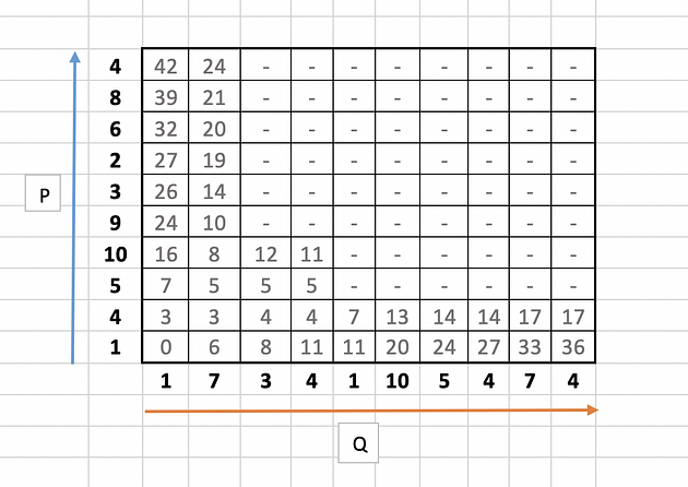
Let us take few examples (11,3 and 8 ) to illustrate the calculation as highlighted in the below table.

for 11,

|10 --4| + min( 5, 12, 5 )
= 6 + 5
= 11
Similarly for 3,
|4 --1| + min( 0 )
= 3+ 0
= 3
and for 8,
|1 --3| + min( 6)
= 2 + 6
= 8
The full table will look like this:

Step 3: Warping Path Identification
Identify the warping path starting from top right corner of the matrix and traversing to bottom left. The traversal path is identified based on the neighbour with minimum value.
In our example it starts with 15 and looks for minimum value i.e. 15 among its neighbours 18, 15 and 18.


The next number in the warping traversal path is 14. This process continues till we reach the bottom or the left axis of the table.

The final path will look like this:


Let this warping path series be called as d.
d = [15,15,14,13,11,9,8,8,4,4,3,0]
Step 4: Final Distance Calculation
Time normalised distance , D


where k is the length of the series d.
k = 12 in our case.
D = ( 15 + 15 + 14 + 13 + 11 + 9 + 8 + 8 + 4 + 4 + 3 + 0 ) /12
= 104/12
= 8.63
Let us take another example with two very similar time series with unit time shift difference.

Cost matrix and warping path will look like this.

DTW distance ,D =
( 0 + 0 + 0 + 0 + 0 +0 +0 +0 +0 +0 +0 ) /11
= 0
Zero DTW distance implies that the time series are very similar and that is indeed the case as observed in the plot.
Resummation (Spaced Repitition)
Dynamic Time Warping (DTW) is a way to compare two -usually temporal- sequences that do not sync up perfectly. It is a method to calculate the optimal matching between two sequences. DTW is useful in many domains such as speech recognition, data mining, financial markets, etc. It's commonly used in data mining to measure the distance between two time-series.
In this post, we will go over the mathematics behind DTW. Then, two illustrative examples are provided to better understand the concept. If you are not interested in the math behind it, please jump to examples.
Formulation
Let's assume we have two sequences like the following:
𝑋=𝑥[1], 𝑥[2], ..., x[i], ..., x[n]
Y=y[1], y[2], ..., y[j], ..., y[m]
The sequences 𝑋 and 𝑌 can be arranged to form an 𝑛-by-𝑚 grid, where each point (𝑖, j) is the alignment between 𝑥[𝑖] and 𝑦[𝑗].
A warping path 𝑊 maps the elements of 𝑋 and 𝑌 to minimize the distance between them. 𝑊 is a sequence of grid points (𝑖, 𝑗). We will see an example of the warping path later.
Warping Path and DTW distance
The Optimal path to (𝑖𝑘, 𝑗𝑘) can be computed by:

where 𝑑 is the Euclidean distance. Then, the overall path cost can be calculated as

Restrictions on the Warping function
The warping path is found using a dynamic programming approach to align two sequences. Going through all possible paths is "combinatorically explosive" [1]. Therefore, for efficiency purposes, it's important to limit the number of possible warping paths, and hence the following constraints are outlined:
Boundary Condition: This constraint ensures that the warping path begins with the start points of both signals and terminates with their endpoints.
Monotonicity condition: This constraint preserves the time-order of points (not going back in time).
Continuity (step size) condition: This constraint limits the path transitions to adjacent points in time (not jumping in time).
In addition to the above three constraints, there are other less frequent conditions for an allowable warping path:
Warping window condition: Allowable points can be restricted to fall within a given warping window of width 𝜔 (a positive integer).
Slope condition: The warping path can be constrained by restricting the slope, and consequently avoiding extreme movements in one direction.
An acceptable warping path has combinations of chess king moves that are:
Horizontal moves: (𝑖, 𝑗) → (𝑖, 𝑗+1)
Vertical moves: (𝑖, 𝑗) → (𝑖+1, 𝑗)
Diagonal moves: (𝑖, 𝑗) → (𝑖+1, 𝑗+1)
Implementation
Let's import all python packages we need.
import pandas as pd import numpy as np# Plotting Packages import matplotlib.pyplot as plt import seaborn as sbn# Configuring Matplotlib import matplotlib as mpl mpl.rcParams['figure.dpi'] = 300 savefig_options = dict(format="png", dpi=300, bbox_inches="tight")# Computation packages from scipy.spatial.distance import euclidean from fastdtw import fastdtw
Let's define a method to compute the accumulated cost matrix D for the warp path. The cost matrix uses the Euclidean distance to calculate the distance between every two points. The methods to compute the Euclidean distance matrix and accumulated cost matrix are defined below:
Example 1
In this example, we have two sequences x and y with different lengths.
Create two sequences\
x = [3, 1, 2, 2, 1] y = [2, 0, 0, 3, 3, 1, 0]
We cannot calculate the Euclidean distance between x and y since they don't have equal lengths.

Example 1: Euclidean distance between x and y (is it possible? 🤔) (Image by Author)
Compute DTW distance and warp path
Many Python packages calculate the DTW by just providing the sequences and the type of distance (usually Euclidean). Here, we use a popular Python implementation of DTW that is FastDTW which is an approximate DTW algorithm with lower time and memory complexities [2].
dtw_distance, warp_path = fastdtw(x, y, dist=euclidean)
Note that we are using SciPy's distance function Euclidean that we imported earlier. For a better understanding of the warp path, let's first compute the accumulated cost matrix and then visualize the path on a grid. The following code will plot a heatmap of the accumulated cost matrix.
cost_matrix = compute_accumulated_cost_matrix(x, y)
Example 1: Python code to plot (and save) the heatmap of the accumulated cost matrix


Example 1: Accumulated cost matrix and warping path (Image by Author)
The color bar shows the cost of each point in the grid. As can be seen, the warp path (blue line) is going through the lowest cost on the grid. Let's see the DTW distance and the warping path by printing these two variables.
DTW distance: 6.0 Warp path: [(0, 0), (1, 1), (1, 2), (2, 3), (3, 4), (4, 5), (4, 6)]
The warping path starts at point (0, 0) and ends at (4, 6) by 6 moves. Let's also calculate the accumulated cost most using the functions we defined earlier and compare the values with the heatmap.
cost_matrix = compute_accumulated_cost_matrix(x, y) print(np.flipud(cost_matrix)) # Flipping the cost matrix for easier comparison with heatmap values!>>> [[32. 12. 10. 10. 6.] [23. 11. 6. 6. 5.] [19. 11. 5. 5. 9.] [19. 7. 4. 5. 8.] [19. 3. 6. 10. 4.] [10. 2. 6. 6. 3.] [ 1. 2. 2. 2. 3.]]
The cost matrix is printed above has similar values to the heatmap.
Now let's plot the two sequences and connect the mapping points. The code to plot the DTW distance between x and y is given below.
Example 1: Python code to plot (and save) the DTW distance between x and y


Example 1: DTW distance between x and y (Image by Author)
Example 2
In this example, we will use two sinusoidal signals and see how they will be matched by calculating the DTW distance between them.
Example 2: Generate two sinusoidal signals (x1 and x2) with different lengths
Just like Example 1, let's calculate the DTW distance and the warp path for *x1 *and *x2 *signals using FastDTW package.
distance, warp_path = fastdtw(x1, x2, dist=euclidean)
Example 2: Python code to plot (and save) the DTW distance between x1 and x2

Example 2: DTW distance between x1 and x2 (Image by Author)
As can be seen in above figure, the DTW distance between the two signals is particularly powerful when the signals have similar patterns. The extrema (maximum and minimum points) between the two signals are correctly mapped. Moreover, unlike Euclidean distance, we may see many-to-one mapping when DTW distance is used, particularly if the two signals have different lengths.
You may spot an issue with dynamic time warping from the figure above. Can you guess what it is?
The issue is around the head and tail of time-series that do not properly match. This is because the DTW algorithm cannot afford the warping invariance for at the endpoints. In short, the effect of this is that a small difference at the sequence endpoints will tend to contribute disproportionately to the estimated similarity[3].
Conclusion
DTW is an algorithm to find an optimal alignment between two sequences and a useful distance metric to have in our toolbox. This technique is useful when we are working with two non-linear sequences, particularly if one sequence is a non-linear stretched/shrunk version of the other. The warping path is a combination of "chess king" moves that starts from the head of two sequences and ends with their tails.
You can find the Jupyter notebook for this blog post here. Thanks for reading!
References
[1] Donald J. Berndt and James Clifford, Using Dynamic Time Warping to Find Patterns in Time Series, 3rd International Conference on Knowledge Discovery and Data Mining
[2] Salvador, S. and P. Chan, FastDTW: Toward accurate dynamic time warping in linear time and space(2007), Intelligent Data Analysis
[3] Diego Furtado Silva, et al., On the effect of endpoints on dynamic time warping (2016), SIGKDD Workshop on Mining and Learning from Time Series
Useful Links
[1] https://nipunbatra.github.io/blog/ml/2014/05/01/dtw.html
[2] https://databricks.com/blog/2019/04/30/understanding-dynamic-time-warping.html
Sounds like time traveling or some kind of future technic, however, it is not. Dynamic Time Warping is used to compare the similarity or calculate the distance between two arrays or time series with different length.
Suppose we want to calculate the distance of two equal-length arrays:
a = [1, 2, 3] b = [3, 2, 2]
How to do that? One obvious way is to match up a and b in 1-to-1 fashion and sum up the total distance of each component. This sounds easy, but what if a and b have different lengths?
a = [1, 2, 3] b = [2, 2, 2, 3, 4]
How to match them up? Which should map to which? To solve the problem, there comes dynamic time warping. Just as its name indicates, to warp the series so that they can match up.
Use Cases
Before digging into the algorithm, you might have the question that is it useful? Do we really need to compare the distance between two unequal-length time series?
Yes, in a lot of scenarios DTW is playing a key role.
Sound Pattern Recognition
One use case is to detect the sound pattern of the same kind. Suppose we want to recognise the voice of a person by analysing his sound track, and we are able to collect his sound track of saying Hello in one scenario. However, people speak in the same word in different ways, what if he speaks hello in a much slower pace like Heeeeeeelloooooo , we will need an algorithm to match up the sound track of different lengths and be able to identify they come from the same person.

Stock Market
In a stock market, people always hope to be able to predict the future, however using general machine learning algorithms can be exhaustive, as most prediction task requires test and training set to have the same dimension of features. However, if you ever speculate in the stock market, you will know that even the same pattern of a stock can have very different length reflection on klines and indicators.
Definition & Idea
A concise explanation of DTW from wiki,
In time series analysis, dynamic time warping (DTW) is one of the algorithms for measuring similarity between two temporal sequences, which may vary in speed. DTW has been applied to temporal sequences of video, audio, and graphics data --- indeed, any data that can be turned into a linear sequence can be analysed with DTW.
The idea to compare arrays with different length is to build one-to-many and many-to-one matches so that the total distance can be minimised between the two.
Suppose we have two different arrays red and blue with different length:

Clearly these two series follow the same pattern, but the blue curve is longer than the red. If we apply the one-to-one match, shown in the top, the mapping is not perfectly synced up and the tail of the blue curve is being left out.
DTW overcomes the issue by developing a one-to-many match so that the troughs and peaks with the same pattern are perfectly matched, and there is no left out for both curves(shown in the bottom top).
Rules
In general, DTW is a method that calculates an optimal match between two given sequences (e.g. time series) with certain restriction and rules(comes from wiki):
Every index from the first sequence must be matched with one or more indices from the other sequence and vice versa
The first index from the first sequence must be matched with the first index from the other sequence (but it does not have to be its only match)
The last index from the first sequence must be matched with the last index from the other sequence (but it does not have to be its only match)
The mapping of the indices from the first sequence to indices from the other sequence must be monotonically increasing, and vice versa, i.e. if
j > iare indices from the first sequence, then there must not be two indicesl > kin the other sequence, such that indexiis matched with indexland indexjis matched with indexk, and vice versa
The optimal match is denoted by the match that satisfies all the restrictions and the rules and that has the minimal cost, where the cost is computed as the sum of absolute differences, for each matched pair of indices, between their values.
To summarise is that head and tail must be positionally matched, no cross-match and no left out.
Implementation
The implementation of the algorithm looks extremely concise:

where DTW[i, j] is the distance between s[1:i] and t[1:j] with the best alignment.
The key lies in:
DTW[i, j] := cost + minimum(DTW[i-1, j ], DTW[i , j-1], DTW[i-1, j-1])
Which is saying that the cost of between two arrays with length i and j equals _the distance between the tails + the minimum of cost in arrays with length *`i-1, j_ , _i, j-1_ , and __i-1, j-1*`_ ._
Put it in python would be:
Example:

The distance between a and b would be the last element of the matrix, which is 2.
Add Window Constraint
One issue of the above algorithm is that we allow one element in an array to match an unlimited number of elements in the other array(as long as the tail can match in the end), this would cause the mapping to bent over a lot, for example, the following array:
a = [1, 2, 3] b = [1, 2, 2, 2, 2, 2, 2, 2, ..., 5]
To minimise the distance, the element 2 in array a would match all the 2 in array b , which causes an array b to bent severely. To avoid this, we can add a window constraint to limit the number of elements one can match:


The key difference is that now each element is confined to match elements in range i --- w and i + w . The w := max(w, abs(n-m)) guarantees all indices can be matched up.
The implementation and example would be:

Apply a Package
There is also contributed packages available on Pypi to use directly. Here I demonstrate an example using fastdtw:
It gives you the distance of two lists and index mapping(the example can extend to a multi-dimension array).

Last updated