DFS
from .all_factors import *
from .count_islands import *
from .pacific_atlantic import *
from .sudoku_solver import *
from .walls_and_gates import *
from .maze_search import *

"""
Numbers can be regarded as product of its factors. For example,
8 = 2 x 2 x 2;
  = 2 x 4.


Write a function that takes an integer n and return all possible combinations
of its factors.Numbers can be regarded as product of its factors. For example,
8 = 2 x 2 x 2;
  = 2 x 4.

Examples:
input: 1
output:
[]


input: 37
output:
[]

input: 32
output:
[
  [2, 16],
  [2, 2, 8],
  [2, 2, 2, 4],
  [2, 2, 2, 2, 2],
"""


def get_factors(n):
    """[summary]

    Arguments:
        n {[int]} -- [to analysed number]

    Returns:
        [list of lists] -- [all factors of the number n]
    """

    def factor(n, i, combi, res):
        """[summary]
        helper function

        Arguments:
            n {[int]} -- [number]
            i {[int]} -- [to tested divisor]
            combi {[list]} -- [catch divisors]
            res {[list]} -- [all factors of the number n]

        Returns:
            [list] -- [res]
        """

        while i * i <= n:
            if n % i == 0:
                res += (combi + [i, int(n / i)],)
                factor(n / i, i, combi + [i], res)
            i += 1
        return res

    return factor(n, 2, [], [])


def get_factors_iterative1(n):
    """[summary]
    Computes all factors of n.
    Translated the function get_factors(...) in
    a call-stack modell.

    Arguments:
        n {[int]} -- [to analysed number]

    Returns:
        [list of lists] -- [all factors]
    """

    todo, res = [(n, 2, [])], []
    while todo:
        n, i, combi = todo.pop()
        while i * i <= n:
            if n % i == 0:
                res += (combi + [i, n // i],)
                todo.append((n // i, i, combi + [i])),
            i += 1
    return res


def get_factors_iterative2(n):
    """[summary]
    analog as above

    Arguments:
        n {[int]} -- [description]

    Returns:
        [list of lists] -- [all factors of n]
    """

    ans, stack, x = [], [], 2
    while True:
        if x > n // x:
            if not stack:
                return ans
            ans.append(stack + [n])
            x = stack.pop()
            n *= x
            x += 1
        elif n % x == 0:
            stack.append(x)
            n //= x
        else:
            x += 1

"""
Given a 2d grid map of '1's (land) and '0's (water),
count the number of islands.
An island is surrounded by water and is formed by
connecting adjacent lands horizontally or vertically.
You may assume all four edges of the grid are all surrounded by water.

Example 1:

11110
11010
11000
00000
Answer: 1

Example 2:

11000
11000
00100
00011
Answer: 3
"""


def num_islands(grid):
    count = 0
    for i in range(len(grid)):
        for j, col in enumerate(grid[i]):
            if col == 1:
                dfs(grid, i, j)
                count += 1
    return count


def dfs(grid, i, j):
    if (i < 0 or i >= len(grid)) or (j < 0 or j >= len(grid[0])):
        return
    if grid[i][j] != 1:
        return
    grid[i][j] = 0
    dfs(grid, i + 1, j)
    dfs(grid, i - 1, j)
    dfs(grid, i, j + 1)
    dfs(grid, i, j - 1)

"""
Find shortest path from top left column to the right lowest column using DFS.
only step on the columns whose value is 1
if there is no path, it returns -1
(The first column(top left column) is not included in the answer.)

Ex 1)
If maze is
[[1,0,1,1,1,1],
 [1,0,1,0,1,0],
 [1,0,1,0,1,1],
 [1,1,1,0,1,1]],
the answer is: 14

Ex 2)
If maze is
[[1,0,0],
 [0,1,1],
 [0,1,1]],
the answer is: -1
"""


def find_path(maze):
    cnt = dfs(maze, 0, 0, 0, -1)
    return cnt


def dfs(maze, i, j, depth, cnt):
    directions = [(0, -1), (0, 1), (-1, 0), (1, 0)]

    row = len(maze)
    col = len(maze[0])

    if i == row - 1 and j == col - 1:
        if cnt == -1:
            cnt = depth
        else:
            if cnt > depth:
                cnt = depth
        return cnt

    maze[i][j] = 0

    for k in range(len(directions)):
        nx_i = i + directions[k][0]
        nx_j = j + directions[k][1]

        if nx_i >= 0 and nx_i < row and nx_j >= 0 and nx_j < col:
            if maze[nx_i][nx_j] == 1:
                cnt = dfs(maze, nx_i, nx_j, depth + 1, cnt)

    maze[i][j] = 1

    return cnt

# Given an m x n matrix of non-negative integers representing
# the height of each unit cell in a continent,
# the "Pacific ocean" touches the left and top edges of the matrix
# and the "Atlantic ocean" touches the right and bottom edges.

# Water can only flow in four directions (up, down, left, or right)
# from a cell to another one with height equal or lower.

# Find the list of grid coordinates where water can flow to both the
# Pacific and Atlantic ocean.

# Note:
# The order of returned grid coordinates does not matter.
# Both m and n are less than 150.
# Example:

# Given the following 5x5 matrix:

# Pacific ~   ~   ~   ~   ~
# ~  1   2   2   3  (5) *
# ~  3   2   3  (4) (4) *
# ~  2   4  (5)  3   1  *
# ~ (6) (7)  1   4   5  *
# ~ (5)  1   1   2   4  *
# *   *   *   *   * Atlantic

# Return:

# [[0, 4], [1, 3], [1, 4], [2, 2], [3, 0], [3, 1], [4, 0]]
# (positions with parentheses in above matrix).


def pacific_atlantic(matrix):
    """
    :type matrix: List[List[int]]
    :rtype: List[List[int]]
    """
    n = len(matrix)
    if not n:
        return []
    m = len(matrix[0])
    if not m:
        return []
    res = []
    atlantic = [[False for _ in range(n)] for _ in range(m)]
    pacific = [[False for _ in range(n)] for _ in range(m)]
    for i in range(n):
        dfs(pacific, matrix, float("-inf"), i, 0)
        dfs(atlantic, matrix, float("-inf"), i, m - 1)
    for i in range(m):
        dfs(pacific, matrix, float("-inf"), 0, i)
        dfs(atlantic, matrix, float("-inf"), n - 1, i)
    for i in range(n):
        for j in range(m):
            if pacific[i][j] and atlantic[i][j]:
                res.append([i, j])
    return res


def dfs(grid, matrix, height, i, j):
    if i < 0 or i >= len(matrix) or j < 0 or j >= len(matrix[0]):
        return
    if grid[i][j] or matrix[i][j] < height:
        return
    grid[i][j] = True
    dfs(grid, matrix, matrix[i][j], i - 1, j)
    dfs(grid, matrix, matrix[i][j], i + 1, j)
    dfs(grid, matrix, matrix[i][j], i, j - 1)
    dfs(grid, matrix, matrix[i][j], i, j + 1)

"""
It's similar to how human solve Sudoku.

create a hash table (dictionary) val to store possible values in every location.
Each time, start from the location with fewest possible values, choose one value
from it and then update the board and possible values at other locations.
If this update is valid, keep solving (DFS). If this update is invalid (leaving
zero possible values at some locations) or this value doesn't lead to the
solution, undo the updates and then choose the next value.
Since we calculated val at the beginning and start filling the board from the
location with fewest possible values, the amount of calculation and thus the
runtime can be significantly reduced:


The run time is 48-68 ms on LeetCode OJ, which seems to be among the fastest
python solutions here.


The PossibleVals function may be further simplified/optimized, but it works just
fine for now. (it would look less lengthy if we are allowed to use numpy array
for the board lol).
"""


class Sudoku:
    def __init__(self, board, row, col):
        self.board = board
        self.row = row
        self.col = col
        self.val = self.possible_values()

    def possible_values(self):
        a = "123456789"
        d, val = {}, {}
        for i in range(self.row):
            for j in range(self.col):
                ele = self.board[i][j]
                if ele != ".":
                    d[("r", i)] = d.get(("r", i), []) + [ele]
                    d[("c", j)] = d.get(("c", j), []) + [ele]
                    d[(i // 3, j // 3)] = d.get((i // 3, j // 3), []) + [ele]
                else:
                    val[(i, j)] = []
        for (i, j) in val.keys():
            inval = (
                d.get(("r", i), []) + d.get(("c", j), []) + d.get((i / 3, j / 3), [])
            )
            val[(i, j)] = [n for n in a if n not in inval]
        return val

    def solve(self):
        if len(self.val) == 0:
            return True
        kee = min(self.val.keys(), key=lambda x: len(self.val[x]))
        nums = self.val[kee]
        for n in nums:
            update = {kee: self.val[kee]}
            if self.valid_one(n, kee, update):  # valid choice
                if self.solve():  # keep solving
                    return True
            self.undo(kee, update)  # invalid choice or didn't solve it => undo
        return False

    def valid_one(self, n, kee, update):
        self.board[kee[0]][kee[1]] = n
        del self.val[kee]
        i, j = kee
        for ind in self.val.keys():
            if n in self.val[ind]:
                if (
                    ind[0] == i
                    or ind[1] == j
                    or (ind[0] / 3, ind[1] / 3) == (i / 3, j / 3)
                ):
                    update[ind] = n
                    self.val[ind].remove(n)
                    if len(self.val[ind]) == 0:
                        return False
        return True

    def undo(self, kee, update):
        self.board[kee[0]][kee[1]] = "."
        for k in update:
            if k not in self.val:
                self.val[k] = update[k]
            else:
                self.val[k].append(update[k])
        return None

    def __str__(self):
        """[summary]
        Generates a board representation as string.

        Returns:
            [str] -- [board representation]
        """

        resp = ""
        for i in range(self.row):
            for j in range(self.col):
                resp += " {0} ".format(self.board[i][j])
            resp += "\n"
        return resp

"""
You are given a m x n 2D grid initialized with these three possible values:
    -1: A wall or an obstacle.
    0: A gate.
    INF: Infinity means an empty room. We use the value 2^31 - 1 = 2147483647 to represent INF
         as you may assume that the distance to a gate is less than 2147483647.
Fill the empty room with distance to its nearest gate.
If it is impossible to reach a gate, it should be filled with INF.

For example, given the 2D grid:
    INF -1  0   INF
    INF INF INF -1
    INF -1  INF -1
    0   -1  INF INF
After running your function, the 2D grid should be:
    3   -1  0   1
    2   2   1   -1
    1   -1  2   -1
    0   -1  3   4
"""


def walls_and_gates(rooms):
    for i in range(len(rooms)):
        for j in range(len(rooms[0])):
            if rooms[i][j] == 0:
                dfs(rooms, i, j, 0)


def dfs(rooms, i, j, depth):
    if (i < 0 or i >= len(rooms)) or (j < 0 or j >= len(rooms[0])):
        return  # out of bounds
    if rooms[i][j] < depth:
        return  # crossed
    rooms[i][j] = depth
    dfs(rooms, i + 1, j, depth + 1)
    dfs(rooms, i - 1, j, depth + 1)
    dfs(rooms, i, j + 1, depth + 1)
dfs(rooms, i, j - 1, depth + 1)Introduction
Depth-First Search - Theory
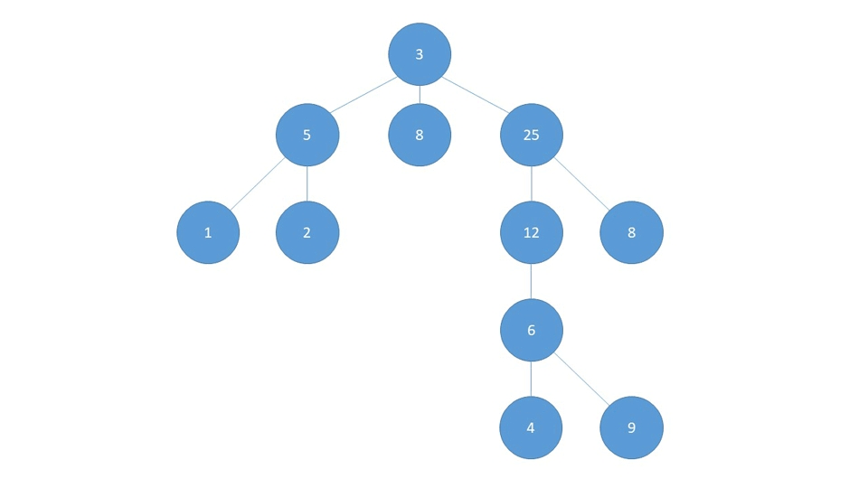
The DFS Algorithm
Depth-First Search - Implementation
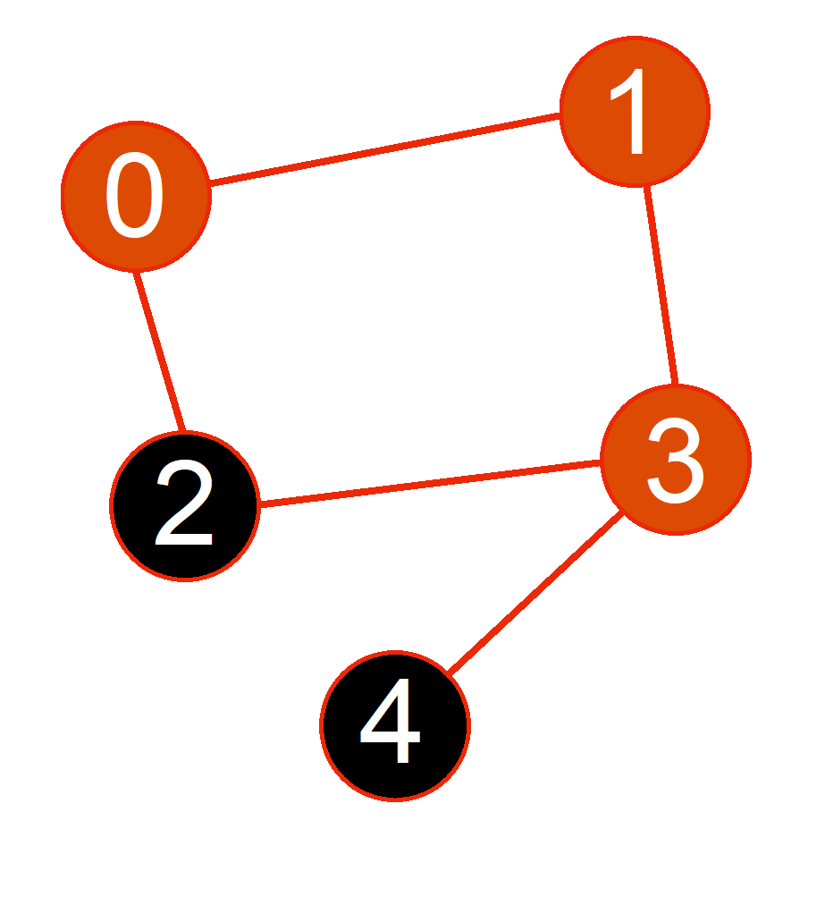
Running DFS
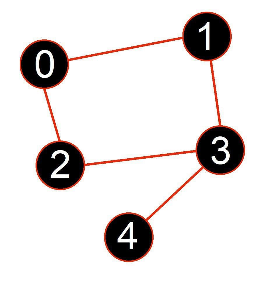
Current Node
Path
Visited
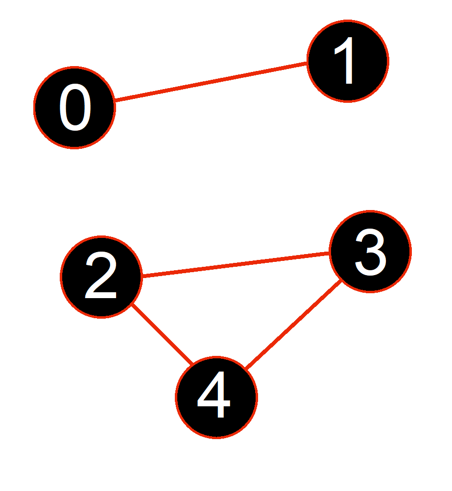
Conclusion
Last updated