Dijkstra's algorithm

Introduction

Dijkstra's algorithm is an algorithm which finds the shortest paths between nodes in a graph. It was designed by a Dutch computer scientist Edsger Wybe Dijkstra in 1956, when he thought about how he might calculate the shortest route from Rotterdam to Groningen. It was published three years later.

In computer science (as well as in our everyday life), there are a lot of problems that require finding the shortest path between two points. We encounter problems such as:

• Finding the shortest path from our house to our school or workplace

• Finding the quickest way to get to a gas station while traveling

• Finding a list of friends that a particular user on social network may know

These are just a few of the many "shortest path problems" we see daily. Dijkstra's algorithm is one of the most well known shortest path algorithms because of it's efficiency and simplicity.

Graphs and Types of Graphs

Dijkstra's algorithm works on undirected, connected, weighted graphs. Before we get into it, let's explain what an undirected, connected, and weighed graph actually is.

A graph is a data structure represented by two things:

• Vertices: Groups of certain objects or data (also known as a "node")

• Edges: Links that connect those groups of objects or data

Let's explain this with an example: We want to represent a country with a graph. That country is made out of cities of different sizes and characteristics. Those cities would be represented by vertices. Between some of those cities, there are roads that connect them. Those roads would be represented by edges.

One more example of a graph can be a circle route of a train: the train stations are represented by vertices, and the rails between them are represented by the edges of a graph.

A graph can even be as abstract as a representation of human relationships: We can represent each person in a group of people as vertices in a graph, and if they know each other, we connect them with an edge.

Graphs can be divided based on the types of their edges or based on the number of components that represent them.

When it comes to their edges, graphs can be:

• Directed

• Undirected

A directed graph is a graph in which the edges have orientations. A second example mentioned above is an example of a directed graph: the train goes from one station to the other, but it can't go in reverse.

An undirected graph is a graph in which the edges do not have orientations (therefore, all edges in an undirected graph are considered to be bidirectional). An example of an undirected graph can be the third example mentioned above: It's impossible for person A to know person B without person B knowing the person A back.

Another division by the edges in a graph can be:

• Weighted

• Unweighted

A weighted graph is a graph whose edges have a certain numerical value joined to them: their weight. For example, if we knew the lengths of every road between each pair of cities in a country, we could assign them to the edges in a graph representation of a country and create a weighted graph. i.e. the weigth or "cost" of an edge is the distance between the cities.

An unweighted graph is a graph whose edges don't have weights, like the forementioned graph of relationships between people - we can't assign a numerical value to "knowing a person"!

Based on the number of components that represent them, graphs can be:

• Connected

• Disconnected

A connected graph is a graph that only consists of one component - every vertex inside of it has a path to every other vertex. If we were at a party, and every person there knew the host, that would be represented with a connected graph - everyone could meet anyone they want via the host.

A disconnected graph is a graph that consists of more than one component. Using the same example, if somehow an outsider who doesn't know anyone ended up at the party, the graph of all people at the party and their relationships, it would now be disconnected, because there is one vertex with no edges to connect it to the other vertices present.

Dijkstra's Algorithm

The original Dijkstra's algorithm finds the shortest path between two nodes in a graph. Another, more common variation of this algorithm finds the shortest path between the first vertex and all of the other vertices in a graph. In this article, we will focus on this variation.

We will now go over this algorithm step by step:

1. First, we will create a set of visited vertices, to keep track of all of the vertices that have been assigned their correct shortest path.

   We will also need to set "costs" of all vertices in the graph (lengths of the current shortest path that leads to it). All of the costs will be set to 'infinity' at the begining, to make sure that every other cost we may compare it to would be smaller than the starting one. The only exception is the cost of the first, starting vertex - this vertex will have a cost of 0, because it has no path to itself.

2. As long as there are vertices without the shortest path assigned to them, we do the following:

   • We pick a vertex with the shortest current cost, visit it, and add it to the visited vertices set

   • We update the costs of all its adjacent vertices that are not visited yet. We do this by comparing its current (old) cost, and the sum of the parent's cost and the edge between the parent (current node) and the adjacent node in question.

Let's explain this a bit better using an example:

graf1

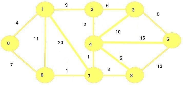
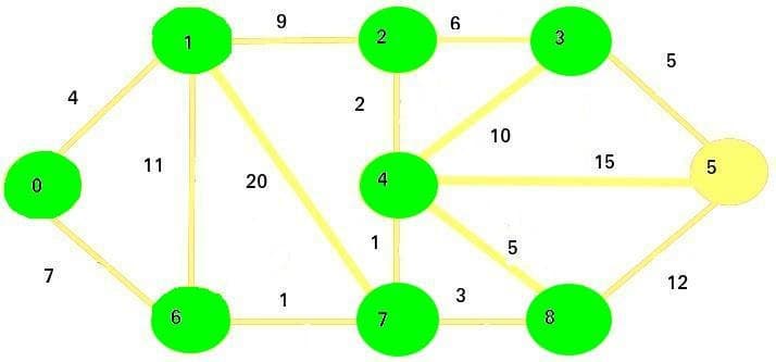
Let's say the vertex 0 is our starting point. We are going to set the initial costs of vertices in this graph like this:

vertex	cost to get to it from vertex 0
0	0
1	inf
2	inf
3	inf
4	inf
5	inf
6	inf
7	inf
8	inf

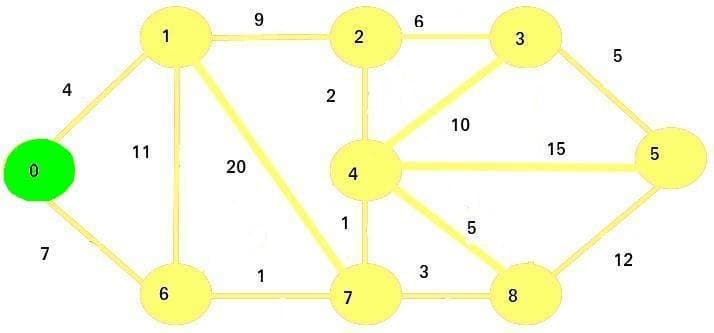
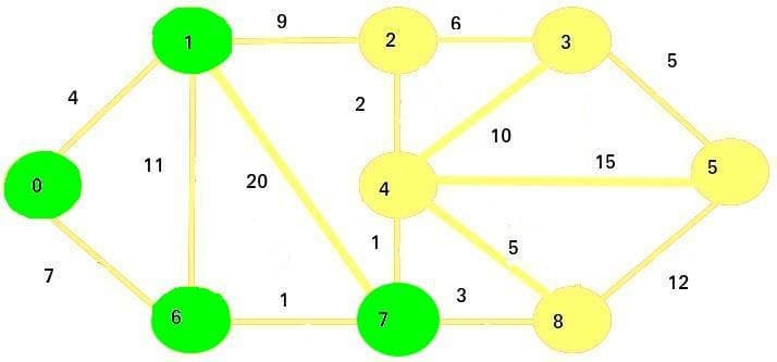
We pick the vertex with a minimum cost - that vertex is 0. We will mark it as visited and add it to our set of visited vertices. The visited nodes will be marked with green color in the images:

graf1

Then, we will update the cost of adjacent vertices (1 and 6).

Since 0 + 4 < infinity and 0 + 7 < infinity, the new costs will be the following (the numbers in bold will be visited vertices):

vertex	cost to get to it from vertex 0
0	0
1	4
2	inf
3	inf
4	inf
5	inf
6	7
7	inf
8	inf

Now we visit the next smallest cost node, which is 1.

graf1

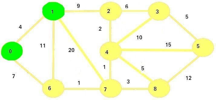
We mark it as visited, and then update the adjacent vertices: 2, 6, and 7:

• Since 4 + 9 < infinity, new cost of vertex 2 will be 13

• Since 4 + 11 > 7, the cost of vertex 6 will remain 7

• Since 4 + 20 < infinity, new cost of vertex 7 will be 24

These are our new costs:

vertex	cost to get to it from vertex 0
0	0
1	4
2	13
3	inf
4	inf
5	inf
6	7
7	24
8	inf

The next vertex we're going to visit is vertex 6. We mark it as visited and update its adjacent vertices' costs:

graf1

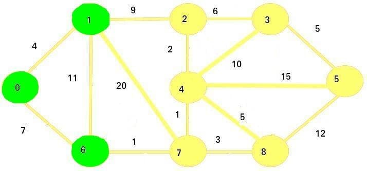
Since 7 + 1 < 24, the new cost for vertex 7 will be 8.

These are our new costs:

vertex	cost to get to it from vertex 0
0	0
1	4
2	13
3	inf
4	inf
5	inf
6	7
7	8
8	inf

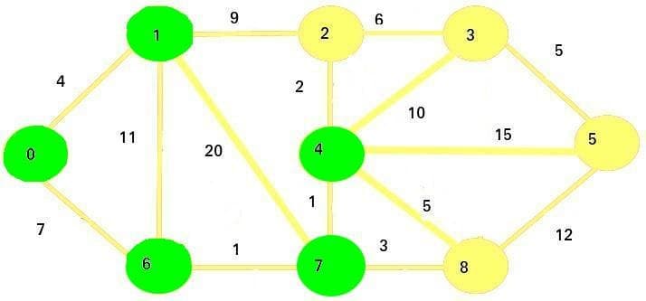
The next vertex we are going to visit is vertex 7:

graf1

Now we're going to update the adjacent vertices: vertices 4 and 8.

• Since 8 + 1 < infinity, the new cost of vertex 4 is 9

• Since 8 + 3 < infinity, the new cost of vertex 8 is 11

These are the new costs:

vertex	cost to get to it from vertex 0
0	0
1	4
2	13
3	inf
4	9
5	inf
6	7
7	8
8	11

The next vertex we'll visit is vertex 4:

graf1

We will now update the adjacent vertices: 2, 3, 5, and 8.

Free eBook: Git Essentials

Check out our hands-on, practical guide to learning Git, with best-practices, industry-accepted standards, and included cheat sheet. Stop Googling Git commands and actually learn it!Download the eBook

• Since 9 + 2 < 13, the new cost of vertex 2 is 11

• Since 9 + 10 < infinity, the new cost of vertex 3 is 19

• Since 9 + 15 < infinity, the new cost of vertex 5 is 24

• Since 9 + 5 > 11, the cost of vertex 8 remains 11

The new costs are:

vertex	cost to get to it from vertex 0
0	0
1	4
2	11
3	19
4	9
5	24
6	7
7	8
8	11

The next vertex we are going to visit is vertex 2:

graf1

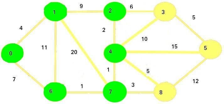
The only vertex we're going to update is vertex 3:

• Since 11 + 6 > 19, the cost of vertex 3 stays the same

Therefore, the current costs for all nodes will stay the same as before.

The next vertex we are going to visit is vertex 8:

graf1

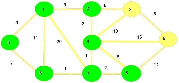
We are updating the vertex 5:

• Since 11 + 12 < 24, the new cost of vertex 5 is going to be 23

The costs of vertices right now are:

vertex	cost to get to it from vertex 0
0	0
1	4
2	11
3	19
4	9
5	24
6	7
7	8
8	11

The next vertex we are going to visit is vertex 3.

graf1

We are updating the remaining adjacent vertex - vertex 5.

• Since 19 + 5 > 23, the cost of vertex 5 remains the same

The final vertex we are going to visit is vertex 5:

graf1

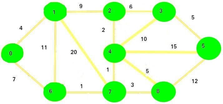
There are no more unvisited vertices that may need an update.

Our final costs represents the shortest paths from node 0 to every other node in the graph:

vertex	cost to get to it from vertex 0
0	0
1	4
2	11
3	19
4	9
5	24
6	7
7	8
8	11

Implementation

Now that we've gone over an example, let's see how we can implement Dijkstra's algorithm in Python!

Before we start, we are first going to have to import a priority queue:

from queue import PriorityQueue

We will use a priority queue to easily sort the vertices we haven't visited yet, which will more easily allow us to choose the one of shortest current cost.

Now, we'll implement a constructor for a class called Graph:

class Graph:

    def __init__(self, num_of_vertices):
        self.v = num_of_vertices
        self.edges = [[-1 for i in range(num_of_vertices)] for j in range(num_of_vertices)]
        self.visited = []

In this simple parametrized constructor, we provided the number of vertices in the graph as an argument, and we initialized three fields:

• v: Represents the number of vertices in the graph

• edges: Represents the list of edges in the form of a matrix. For nodes u and v, self.edges[u][v] = weight of the edge

• visited: A set which will contain the visited vertices

Now, let's define a function which is going to add an edge to a graph:

    def add_edge(self, u, v, weight):
        self.edges[u][v] = weight
        self.edges[v][u] = weight

Now, let's write the function for Dijkstra's algorithm:

    def dijkstra(self, start_vertex):
        D = {v:float('inf') for v in range(self.v)}
        D[start_vertex] = 0

        pq = PriorityQueue()
        pq.put((0, start_vertex))

        while not pq.empty():
            (dist, current_vertex) = pq.get()
            self.visited.append(current_vertex)

            for neighbor in range(self.v):
                if self.edges[current_vertex][neighbor] != -1:
                    distance = self.edges[current_vertex][neighbor]
                    if neighbor not in self.visited:
                        old_cost = D[neighbor]
                        new_cost = D[current_vertex] + distance
                        if new_cost < old_cost:
                            pq.put((new_cost, neighbor))
                            D[neighbor] = new_cost
        return D

In this code, we first created a list D of the size v. The entire list is initialized to infinity. This is going to be a list where we keep the shortest paths from start_vertex to all of the other nodes.

We set the value of the start vertex to 0, since that is its distance from itself.

Then, we initialize a priority queue, which we will use to quickly sort the vertices from the least to most distant. We put the start vertex in the priority queue.

Now, for each vertex in the priority queue, we will first mark them as visited, and then we will iterate through their neighbors.

If the neighbor is not visited, we will compare its old cost and its new cost.

The old cost is the current value of the shortest path from the start vertex to the neighbor, while the new cost is the value of the sum of the shortest path from the start vertex to the current vertex and the distance between the current vertex and the neighbor.

If the new cost is lower than the old cost, we put the neighbor and its cost to the priority queue, and update the list where we keep the shortest paths accordingly.

Finally, after all of the vertices are visited and the priority queue is empty, we return the list D. Our function is done!

Let's put the graph we used in the example above as the input of our implemented algorithm: